Ask Your Question
2

help with graphics_array magic, please

asked 2019-04-15 23:25:48 +0200

stockh0lm gravatar image

updated 2019-04-16 21:57:22 +0200

FrédéricC gravatar image

following Juanjo's advice, I created a graphics_array.

Because i want to do a pairwise comparison with my graphs, i reordered them (with the zip). Now i have a 2xn array, with all the same x- and y-axis lables and also the same leged_labels, so I want to make it nice and put the legend_lable just in the bottom right plot and the left row gets the y-axis lable and the bottom row the x-axis lable.

here is my attempt at doing that.

l = []
k=1.0
p=plot(k*sin(x),(x,-pi,pi),axes_labels=['','$\\varphi$ in [V]'])
l.append(p)
k+=1
p=plot(k*sin(x),(x,-pi,pi))
l.append(p)
k+=1
p=plot(k*sin(x),(x,-pi,pi),axes_labels=['$z_c$ in [m]','$\\varphi$ in [V]'])
l.append(p)
k+=1
p=plot(k*sin(x),(x,-pi,pi), legend_label=['text'],axes_labels=['$z_c$ in [m]',''])
l.append(p)

ym = 1e+20
yM = 1e-20
for i in range(len(l)):
    bounds = l[i].get_minmax_data()
    ym = min(ym, bounds["ymin"])
    yM = max(yM, bounds["ymax"])

gpairs = list(zip(l[::2], l[1::2]))

pic=graphics_array(gpairs) # each plot uses its own vertical scale
graphics_array(gpairs).show(ymin=ym,ymax=yM, frame=True,figsize=[4,8],gridlines=True,typeset='latex',) # same scale for all plots
pic.save('pairwise-comp

This is the pic i get: image description

The labels on the y-axes are gone. only the bottom right has the x-axis lable. and the legend_lable is double in the bottom right.

I have not tried to decorate the rows with text left to the graphs and columns above the graphs.

is what i try to do feasable? or how can i do those things in LaTeX, outside sage? I dont see how i could do the ymin,ymax scaling in latex, but i could do that manually in sage and go back to individual graphs, if all else fails.

edit retag flag offensive close merge delete

Comments

3 Answers

Sort by » oldest newest most voted
4

answered 2019-04-16 06:25:43 +0200

dsejas gravatar image

updated 2019-04-16 22:19:00 +0200

Hello, again, @stockh0lm. You post questions that are really challenging; this one took me various hours. Most of the things that you want to do, Sage does not do by default (I think). You must be doing an amazing research! I had to extract a bit of code from SageMath, and modify it, but this will do the trick.

We will start by creating the plots you need, and wrapping them inside a list 'l':

l = []
k = 1.0
p = plot(k*sin(x),(x,-pi,pi), legend_label='text')
l.append(p)
k += 1
p = plot(k*sin(x),(x,-pi,pi))
l.append(p)
k += 1
p = plot(k*sin(x),(x,-pi,pi))
l.append(p)
k += 1
p = plot(k*sin(x),(x,-pi,pi))
l.append(p)

Notice I have used the legend_label option in the first plot, because putting it in any other of the plots, causes duplicated legends (really don't know why, but it seems to be related to the way SageMath interfaces with Matplotlib).

Now, we are going to convert the plots to Matplotlib format with the following code:

import matplotlib.pyplot as mpl
fig = mpl.figure()
for i, g in zip(range(1, 5), pic._glist):
    subplot = mpl.subplot(2, 2, i)
    # All plots use the same $y$ scale:
    g.matplotlib(figure=fig, sub=subplot, verify=True, axes=True, frame=True, ymin=ym, ymax=yM, gridlines='major')

This is basically the code at the heart of the subroutine that plots a graphics_array (similiar to our variable l), so nothing extra has been added so far. The meaning of almost every sentence here can be deduced from my previous answer, but the important part is we are using your ym and yM as our ymin and ymax, respectively.

The new thing we are going to add is the following:

fig.text(0.5, 0.0, '$z_c$ in [m]', horizontalalignment='center', fontsize=15)
fig.text(0.0, 0.5, '$\\varphi$ in [V]', horizontalalignment='center', rotation=90, fontsize=15)

These are simple text drawing subroutines from Matplotlib. We are telling to add the text to the figure represented by fig, which we created before. Did you notice the coordinates I used? They are absolute coordinates, i.e., they are normalized from 0 to 1. So, when I say 0.5, 0.0 in the first text() command, I am indicating the center of the $x$- axis. The horizontal alignment='center'argument tells Matplotlib center the text at this point. The rotation (in the second text() command) and fontsize options are self-explaining.

Now we save the plot:

g.save('test.png', figure=fig, sub=subplot, verify=True, axes=True, frame=True)

You may have noticed that I indicated axes=True, frame=True in the first chunk of code as in this last line. I don't know why, but if you exclude one of them, the results are quite strange. For example, deleting these options in the last line draws axes and frames for the first 3 plots, but the last one only has axes. Maybe somebody more experienced with SageMath (or more intelligent) than me can explain this.

Anyway, the result should look like this: image description

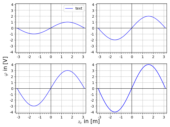
As always, I add a permalink to a Sage Cell with the corresponding code.

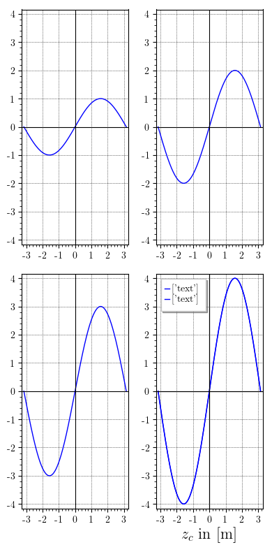
Update: I just found a way of putting the legend on the lower right plot, so I am posting it as an alternative. What you have to do is to use the legend_label=None option for the plot commands when creating the list l:

l = []
k = 1.0
p = plot(k*sin(x),(x,-pi,pi), legend_label=None)
l.append(p)
k += 1
p = plot(k*sin(x),(x,-pi,pi), legend_label=None)
l.append(p)
k += 1
p = plot(k*sin(x),(x,-pi,pi), legend_label=None)
l.append(p)
k += 1
p = plot(k*sin(x),(x,-pi,pi), legend_label=None)
l.append(p)

Once done this, you just have to add the following code after the for loop:

ax = fig.gca()
ax.legend(labels=['text'])

That's it! Here is the result: image description 
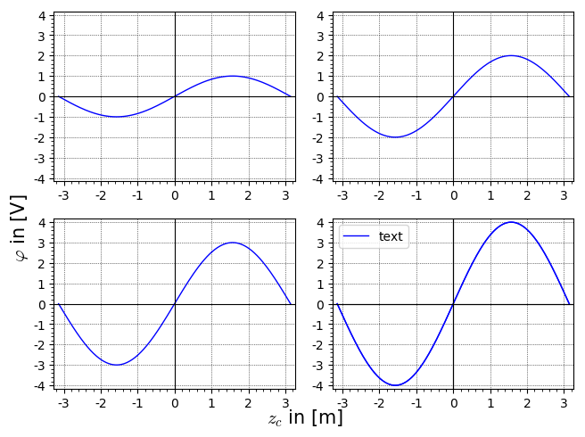
and here is the corresponding code.

Happy to help! Sorry for the long answer!

edit flag offensive delete link more

Comments

amazing, thank you for putting in so much time and effort! And the result is great. Can you explain the double legend in the bottom right pic? it should have only one, right?

stockh0lm gravatar imagestockh0lm ( 2019-04-16 07:30:09 +0200 )edit

Curious indeed. My guess is that Sage has to plot various graphs, so at some point it assumes there are more than one, and adds two legends. This theory seems correct since putting the legend on the first plot, makes just one legend. Is it too important to put it on the last plot?

dsejas gravatar imagedsejas ( 2019-04-16 08:05:11 +0200 )edit

no, first plot is just fine, too. as long as its there and correct. :-)

stockh0lm gravatar imagestockh0lm ( 2019-04-16 08:22:37 +0200 )edit

I have adapted my answer to put the legend in the first plot. I imagine this solves your problems with this particular graphic.

dsejas gravatar imagedsejas ( 2019-04-16 09:44:59 +0200 )edit

I don't believe this, but I just found a way to put the legend on the lower right plot. I am adding it to my answer right now. Unbelievable!!!

dsejas gravatar imagedsejas ( 2019-04-16 09:50:30 +0200 )edit
3

answered 2019-04-16 03:22:58 +0200

Juanjo gravatar image

updated 2019-04-16 03:34:48 +0200

Check the following example:

# Construct the list of plots
p = []
nplots = 8 # number of plots
for i in range(nplots):
    plt = plot([random()*sin(x),random()*cos(x)],(x,-pi,pi), 
               color=["red","green"],legend_label=['sin','cos'])
    plt.legend(False) # don't display legends
    p.append(plt)

# Get ymin and ymax
ym = 1e+20
yM = 1e-20
for i in range(nplots):
    bounds = p[i].get_minmax_data()
    ym = min(ym, bounds["ymin"])
    yM = max(yM, bounds["ymax"])

# Display legends in the penultimate plot
p[-2].legend(True)

# Label the plots on the left column
for i in range(0,nplots-2,2):
    p[i].axes_labels(["",r"$\varphi$ in [V]"])

# Label the plots in the last row
p[-2].axes_labels(["$z_c$ in [m]",r"$\varphi$ in [V]"])
p[-1].axes_labels(["$z_c$ in [m]",""])

# Show plots
ga = graphics_array(p,nrows=nplots/2,ncols=2)
ga.show(ymin=ym,ymax=yM,frame=True, figsize=[8,10])

I think it satisfies almost all your requirements. Since labels are doubled if printed in the bottom right plot (I don't know why), I have included them in the bottom left plot.

Note to Sage developers: I think there is a bug in the definition of graphics_array. If only the optional argument ncols is given, the other dimension, i.e. nrows is not always correctly computed (same thing if only nrows is given). For example, let us consider the code:

ga = graphics_array([plot(sin)] * 6, ncols=2)
ga.show(frame=True)
ga.nrows(), ga.ncols()

This yields (4,2) and an array of 8 plots, the last two ones showing an empty frame. However, one could reasonably expect 6 plots arranged in 3 rows and 2 columns.

Edit: This is the graphics I get for the first example image description

edit flag offensive delete link more

Comments

thank you very much, this is awesome!

stockh0lm gravatar imagestockh0lm ( 2019-04-16 07:31:37 +0200 )edit
0

answered 2020-12-21 23:07:42 +0200

rhymesayers gravatar image

updated 2020-12-22 00:15:22 +0200

@dsejas Thank you for all the work done above. But, if I wanted to add a title to each of the subplots, how would I go about doing this through matplotlib? I figured out how to do it through sage and @Juanjo 's way, but wondering if I can do it through python? Thanks again

edit flag offensive delete link more

Comments

1

Hello, @rhymesayers! If you don't mind, perhaps you could post this as a separate question, so that other users with the same problem can find it quickly. Meanwhile, here is a quick answer: You can use the subplot.title.set_text() command to add a title to each subplot. Concretely, right after the line subplot = mpl.subplot(2, 2, i) (line 25 of my code), you can add subplot.title.set_text('Plot ' + str(i)) in order to add titles like "Plot 1", "Plot 2", etc.

dsejas gravatar imagedsejas ( 2020-12-21 23:43:12 +0200 )edit
1

Yes, please make this a new question.

slelievre gravatar imageslelievre ( 2020-12-22 06:48:51 +0200 )edit

Your Answer

Please start posting anonymously - your entry will be published after you log in or create a new account.

Add Answer

Question Tools

2 followers

Stats

Asked: 2019-04-15 23:25:48 +0200

Seen: 804 times

Last updated: Dec 22 '20