I wonder if there is not a little display bug inside the Sagemath SageMath
linear program since the display of the result here is given given
before the display of the program (for some other programs programs
it is given inside).
nmd= 10 #nombre # Nombre de contraintes
mmd= 6 #nombre contraintes et de variables
Amd= matrix(nmd,mmd,[250,770,360,190,230,-1,0,0,0,0,0,1,31,44,14,27,3,0,480,1770,800,580,160,0, 1,0,0,0,0,0, 0,1,0,0,0,0, 0,0,1,0,0,0, 0,0,0,1,0,0, 0,0,0,0,1,0, 0,0,0,0,0,1]) #les coefficients variables.
nmd, mmd = 10, 6
# Coefficients pour chaque contraintes
bmdmin=[0,600,30,0,0,0,0,0,0] #les bornes contrainte.
coeffs = [(250, 770, 360, 190, 230, -1),
          (0, 0, 0, 0, 0, 1),
          (31, 44, 14, 27, 3, 0),
          (480, 1770, 800, 580, 160, 0),
          (1, 0, 0, 0, 0, 0),
          (0, 1, 0, 0, 0, 0),
          (0, 0, 1, 0, 0, 0),
          (0, 0, 0, 1, 0, 0),
          (0, 0, 0, 0, 1, 0),
          (0, 0, 0, 0, 0, 1)]
# Matrice des contraintes.
Amd = matrix(nmd, mmd, coeffs)
# Bornes inférieures pour les contraintes
bmdmax=[0,900,1000,Infinity,Infinity,Infinity,Infinity,Infinity,Infinity,Infinity] #les bornes contraintes.
bmdmin = [0, 600, 30, 0, 0, 0, 0, 0, 0]
# Bornes supérieures pour les  contraintes (oo=infini)
show(LatexExpr("A="),A1)
show(LatexExpr("bmin="),bmdmin)
show(LatexExpr("bmax="),bmdmax)
md=MixedIntegerLinearProgram(maximization=False, solver="GLPK",) #on (oo = infini).
bmdmax = [0, 900, 1000, oo, oo, oo, oo, oo, oo, oo]
# Visualisons.
show(LatexExpr("A="), Amd)
show(LatexExpr("bmin="), bmdmin)
show(LatexExpr("bmax="), bmdmax)
# On crée le programme de maximization
x=md.new_variable(integer=False,nonnegative=True, indices=[0..mmd-1]) #les nouvelles maximisation.
md = MixedIntegerLinearProgram(maximization=False, solver="GLPK")
# Nouvelles variables: x_0 ... x_2; 'integer' dit si variables sont x_0...x_2 #integer=nombre entier
Bmd=Amd*x #la fonction à valeurs entières
x = md.new_variable(integer=False, nonnegative=True, indices=[0 .. mmd - 1])
# Fonction linéaire pour les contraintes
md.set_objective(1.2*x[0]+4.5*x[1]+3.7*x[2]+6.3*x[3]+3.2*x[4]) # contraintes.
Bmd = Amd * x
# On fixe l'objectif
#on l'objectif.
md.set_objective(1.2*x[0] + 4.5*x[1] + 3.7*x[2] + 6.3*x[3] + 3.2*x[4])
# On construit les contraintes avec leurs bornes
bornes.
for i in range(0,4):
    md.add_constraint(Bmd[i], min=bmdmin[i], max=bmdmax[i])
md.show()
md.solve()
md.get_values(x)
xmd=md.get_values(x)
xmd = md.get_values(x)
# Le résultat.
show(xmd)
Output:
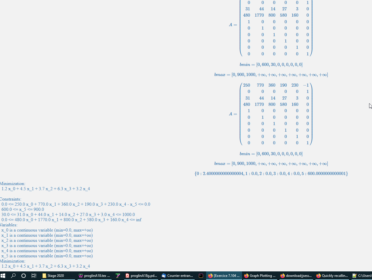
𝐴=(...)

𝑏𝑚𝑖𝑛=[0,600,30,0,0,0,0,0,0]

𝑏𝑚𝑎𝑥=[0,900,1000,+∞,+∞,+∞,+∞,+∞,+∞,+∞]

Minimization:
  1.2 x_0 + 4.5 x_1 + 3.7 x_2 + 6.3 x_3 + 3.2 x_4

Constraints:
  0.0 <= 250.0 x_0 + 770.0 x_1 + 360.0 x_2 + 190.0 x_3 + 230.0 x_4 - x_5 <= 0.0
  600.0 <= x_5 <= 900.0
  30.0 <= 31.0 x_0 + 44.0 x_1 + 14.0 x_2 + 27.0 x_3 + 3.0 x_4 <= 1000.0
  0.0 <= 480.0 x_0 + 1770.0 x_1 + 800.0 x_2 + 580.0 x_3 + 160.0 x_4 <= inf
Variables:
  x_0 is a continuous variable (min=0.0, max=+oo)
  x_1 is a continuous variable (min=0.0, max=+oo)
  x_2 is a continuous variable (min=0.0, max=+oo)
  x_3 is a continuous variable (min=0.0, max=+oo)
  x_4 is a continuous variable (min=0.0, max=+oo)
  x_5 is a continuous variable (min=0.0, max=+oo)

{0:2.4000000000000004,1:0.0,2:0.0,3:0.0,4:0.0,5:600.0000000000001}
Of course I am aware that without the show() command there is no problem. But, for uniformity of presentation I need this command. As I could call it in an other cell the problem an be circonvened. circumvented. But for economic reasons I would prefer to have the code and the result in the same cell. Nevertheless, this is just a remark.