Ask Your Question
2

Problem with implicit_plot

asked 2020-05-18 09:30:23 +0200

jga gravatar image

updated 2020-05-20 11:42:58 +0200

I have three huge degree 31 bivariate polynomials (20,000 characters long each) I want to plot, but I keep getting a lot of noise in my plot. I can't upload it, but the point is that in some regions I just get colorful noise. I've tried defining the polynomials over RealField(n) and increasing the number of plot_points, but neither of these approaches work. Any ideas on how to work around this? Thanks.

Edit: Tried using sympy's plot_implicit and it's so (SO!) slow. Then used numpy's contour_plot and it's fast, but has the same problem as sage.

Here's the code that produces the polynomials and plot. Be patient as it could be a bit slow (depending on your machine).

plot = Graphics()
m = 32-1
D = [(i,j) for i in range(0,m+1) for j in range(0,m+1) if i+j<m+1]

#Polygon
P = Polyhedron( vertices= [(0, 0), (32, 44), (23, 0), (10, 14), (2, 3)] )
points = P.integral_points()

plot_pts = point(points, rgbcolor=(0, 0, 0), size = 20).plot()
plot_np = P.plot(fill = False, point=False, line='black')

M = matrix(ZZ, len(points), len(D), 0)

for row_num, row in enumerate(points):
    for col_num, column in enumerate(D):
        i, j = row
        a, b= column
        #Matrix for interpolation:
        M[row_num, col_num] = (i^a)*(j^b) 

R = PolynomialRing(QQ, 2, 'xy') 
S = PolynomialRing(RealField(500), 2, 'uv') 
x, y = R.gens()       
u, v = S.gens() 
K = M.right_kernel() 
Kdim = K.dimension() 
print(Kdim) 
if Kdim > 0: 
     for l in range(Kdim): 
        K_basis = K.basis()[l] 
        #Writing the interpolating polynomial 
        f=0 
        for order, bidegree in enumerate(D): 
            a, b = bidegree 
            f += list(K_basis)[order] * u^a * v^b 
        F = f.factor()
        f = F[6][0]

        cols = ['red', 'blue', 'green'] 
        interpolation = implicit_plot(f, (u,-1,34), (v,-1,45), plot_points=100, color=cols[l]) 
        plot += interpolation 
plot += plot_pts + plot_np 
plot.show(figsize=10)

Edit 2: Using the mpmath library in Python and with the aid of Sébastien's code below I wrote a routine that allows us to control the root finding method and precision of our computations. I tried several methods, secant (default), newton, hailley, mnewton, etc. without success. Changing the precision and tolerance of the root finding function from mpmath didn't help either. I think this polynomial just behaves too wildly in the region of the plot.

Here's the code and relevant documentation for the "mpmath.findroot" function:

http://mpmath.org/doc/current/calculu... :

from sympy import *
import matplotlib.pyplot as plt
import mpmath as mp

mp.dps = 100
stepx = 0.1
stepy = 0.5
xrange = np.arange(7.5,12.5, stepx)
yrange = np.arange(0, 5, stepy)

def plot_roots_of_f(f):
    L = []
    for u in xrange:
        for v in yrange:
            Root = mp.findroot(f.eval({x:u}),v, method = 'mnewton', tol = E-60, verbose=False,verify=False)
            L.append([u,Root])
    return plt.plot(*zip(*L),linestyle='None', marker='.')

plot_roots_of_f(f)
plt.show()
edit retag flag offensive close merge delete

Comments

Could you please try to upload the code somewhere so taht we can give a try ?

tmonteil gravatar imagetmonteil ( 2020-05-18 19:11:28 +0200 )edit

I added the code, @tmonteil

jga gravatar imagejga ( 2020-05-19 00:42:34 +0200 )edit

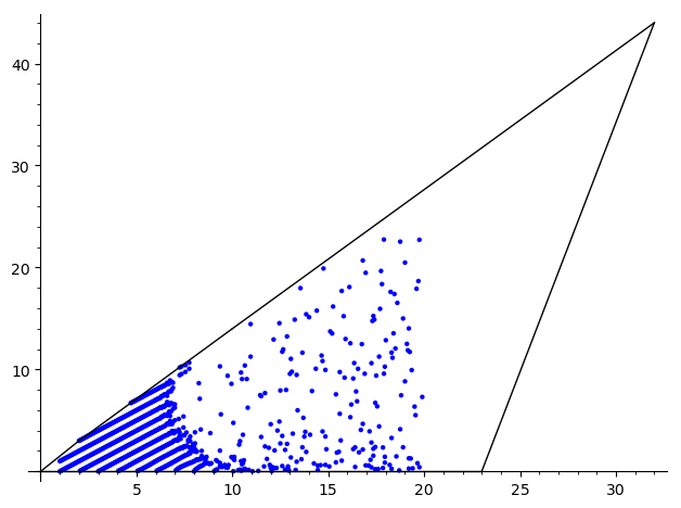
The code runs in few seconds on my machine (does not seem computationally heavy?). The output is the overlay the three implicit plot which indeed looks like "colorful noise". But what is the expected result? Is the equation f==0 suppose to pass through all of the integer points inside the polygon?

Sébastien gravatar imageSébastien ( 2020-05-19 09:41:34 +0200 )edit

@Sébastien exactly. These three polynomials should define nice graphs passing through said points.This must be the case because for each fixed value of x there can be at most 31 values of y in the plot. These vary continuously as x does, so there's just no way it looks as the plot suggests. In my case this is very clear for x<10, where the plot looks well. The issue happens further away from the origin.

jga gravatar imagejga ( 2020-05-19 10:15:44 +0200 )edit
1

I think the generic implicit_plot function is no good for your function f which involves sums of large numbers (possibly done with using float inputs) that must equal to zero at the end. I would suggest you to write your own drawing function based on factorization of the univariate polynomial f after evaluation at specific values of u. For example:

sage: f.subs(u=14.7).factor()
(-1.02680916303147e30) * (v - 10.0971622442134) * (v - 2.04438249413817) * (v + 1.88294590341942) * (v + 12.3103608056188) * (v + 29.6136637586803) * (v^2 - 56.4157620800683*v + 804.755073557794) * (v^2 - 50.4692924243472*v + 691.858754703194) * (v^2 - 44.2941922218622*v + 606.707600654288) * (v^2 - 33.9849183617846*v + 477.330795667438) * (v^2 - 21.5731314846998*v + 318.8705...) * (v^2 - 10.1....)
Sébastien gravatar imageSébastien ( 2020-05-19 13:53:18 +0200 )edit

1 Answer

Sort by » oldest newest most voted
1

answered 2020-05-19 14:12:22 +0200

Sébastien gravatar image

updated 2020-05-20 09:13:15 +0200

It seems that the polynomial f itself does not contain the good information.

sage: f.parent()
Multivariate Polynomial Ring in u, v over Real Field with 500 bits of precision

Because when I draw its roots with:

def roots_of_f(start,stop,step):
    u_range = srange(start, stop, step)
    L = [(u,v) for u in u_range 
               for v in f.subs(u=u).univariate_polynomial().roots(multiplicities=False) 
               if (u,v) in P]
    return L

I get (points is a list in the code and overwrites the sage function points, so I am using point below):

sage: point(roots_of_f(1,20,.05)) + plot_np

image description

Replacing u and v by x and y to use the ring over the rational field seems to give the same thing.

sage: R
Multivariate Polynomial Ring in x, y over Rational Field

Are you sure about that polynomial f ? because the following seems weird:

sage: f.subs(u=20)
0
edit flag offensive delete link more

Comments

1

Thanks for your reply! The polynomials are not irreducible and contain the 6 vertical lines x=19,20,21,22,23,24. I've added two lines in the original code to get rid of them. From what you wrote it seems like the issue goes all the way down to the "roots" algorithm. I gather this method relies on "Brent's method", which requires some kind of regularity from the function. Presumably these polynomials don't satisfy the required hypotheses. I will try to see if manually implementing some other root finding algorithms could help.

jga gravatar imagejga ( 2020-05-19 23:18:13 +0200 )edit
1

I replaced the function draw_roots_of_f in the answer by a function roots_of_f to return a list of roots. This allows me to verify the output of the roots finding algorithm. The following looks ok:

sage: L = roots_of_f(4,5,1)
sage: L
[(4, 5), (4, 4), (4, 3), (4, 2), (4, 1), (4, 0)]
sage: max(abs(f(uv)) for uv in L)
0

But, I agree that the following is weird:

sage: L = roots_of_f(4,5,.5)
sage: max(abs(f(uv)) for uv in L)
8.89546321071247e49

In fact the roots returned by roots_of_f are not precise enough:

sage: f(4,2)
0
sage: f(4,2.00000015504052)
8.65952734939081e46
Sébastien gravatar imageSébastien ( 2020-05-20 09:19:23 +0200 )edit

Thank you, @Sébastien. I think what we're seeing is just a more contrived version of this: https://en.wikipedia.org/wiki/Wilkins... . Your latest experiments also point in this direction. I also did some experiments on my side, please see the original post for the code and a brief summary. I'm also accepting this answer because it provided a solid explanation as to why every method fails. Specially the last comment showing the instability.

jga gravatar imagejga ( 2020-05-20 11:35:19 +0200 )edit

Your Answer

Please start posting anonymously - your entry will be published after you log in or create a new account.

Add Answer

Question Tools

1 follower

Stats

Asked: 2020-05-18 09:30:23 +0200

Seen: 472 times

Last updated: May 20 '20