Ask Your Question
2

Plot solutions of two differential equations on same axes with legend

asked 2020-03-27 21:59:50 +0100

PolarizedIce gravatar image

updated 2021-03-21 00:17:51 +0100

slelievre gravatar image

I need to plot two differential equations on the same set of axes (with a legend showing which is which).

My domain has to be 0 ≤ t ≤ 100.

Listed below is my code, any help is greatly appreciated.

t = var('t')
x = function('x')(t)
y = function('y')(t)
de1 = diff(x,t) == -3/20*x + 1/12*y
de2 = diff(y,t) == 3/20*x-3/20*y
sol = desolve_system([de1,de2],[x,y],ics=[0,4,0])

f(t) = sol[0].rhs()
g(t) = sol[1].rhs()
edit retag flag offensive close merge delete

Comments

What do you mean by "plot" a differential equation? Do you mean plot the solution? Plot a vector field?

John Palmieri gravatar imageJohn Palmieri ( 2020-03-27 22:36:40 +0100 )edit
John Palmieri gravatar imageJohn Palmieri ( 2020-03-27 22:39:35 +0100 )edit

Yes, sorry for the lack of clarity, but I'm meaning to plot the solutions of de1 and de2 at the same time. Thank you for the link.

PolarizedIce gravatar imagePolarizedIce ( 2020-03-28 02:56:46 +0100 )edit

2 Answers

Sort by » oldest newest most voted
6

answered 2020-03-28 01:07:14 +0100

dsejas gravatar image

updated 2020-03-29 16:30:38 +0100

Hello, @PolarizedIce! If what you mean by "plot a differential equation" is "plot it's solution", your code is really close. You can do the following:

t = var('t')
x = function('x')(t)
y = function('y')(t)
de1 = diff(x,t) == -3/20*x + 1/12*y
de2 = diff(y,t) == 3/20*x-3/20*y
sol = desolve_system([de1,de2],[x,y],ics=[0,4,0])

f(t) = sol[0].rhs()
g(t) = sol[1].rhs()

p  = plot(f, (t, 0, 100), color='red')
p += plot(g, (t, 0, 100), color='blue')
p.show()

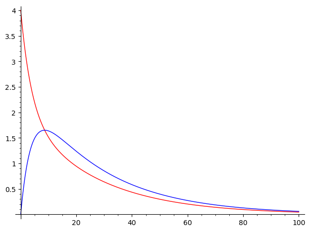
Here, I used the color option just to make clear which function is which. You can also plot both functions at the same time:

plot([f,g], (t,0,100))

As an alternative, in this particular case, you can also use the desolve_system_rk4 function:

t,x,y = var('t x y')
de1 = -3/20*x + 1/12*y
de2 = 3/20*x-3/20*y
sol = desolve_system_rk4([de1,de2], [x,y], ivar=t, ics=[0,4,0], end_points=100)

Notice that the differential equations must be of the form $\frac{dx}{dt}=F(x,t)$, so you use only the right-hand-side of your equations (see de1 and de2 in the previous code). Once you have specified the rhs of the equations, you specify the dependent variables, the independent variable, the initial condition, and finally, you introduce the final point of integration (I chose 10 in this case). You can also specify a step of integration with the step option (the default is step=0.1) . I must point out that desolve_system_rk4 solves the system numerically, as opposed to desolve_system, that solves symbolically.

In order to plot the numerical solution, you can do the following:

f = [(i,j) for i,j,k in sol]
g = [(i,k) for i,j,k in sol]
p = line(f, color='red')
p += line(g, color='blue')
p.show()

Whichever method you use, this should be the result: image description
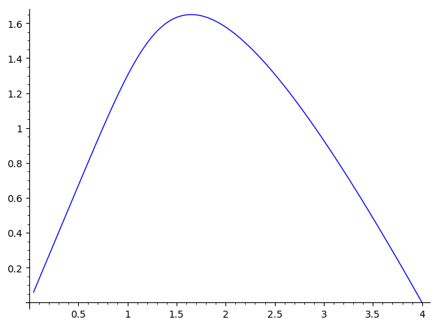
On the other hand, you can also plot the phase portrait. If you used the desolve_system, you should do

fp = [(f(t),g(t)) for t in srange(0,100,0.1)]
line(fp)

If you used desolve_system_rk4, then you should do

fp = [(j,k) for i,j,k in sol]
line(fp)

Whatever method you used, the result should be like this: image description
I hope this helps!

edit flag offensive delete link more

Comments

Hello, @PolarizedIce! I just noticed that you wanted your domain to be $0\le t\le 100$. My previous answer worked one example in $0\le t\le 10$. So I have updated my answer to work with your required domain. The only difference is that I changed end_points=10 to end_points=100 in the command desolve_system_rk4, and the first figure has changed in consequence; everything else remains the same.

dsejas gravatar imagedsejas ( 2020-03-28 17:50:13 +0100 )edit
5

answered 2020-03-28 04:38:19 +0100

Juanjo gravatar image

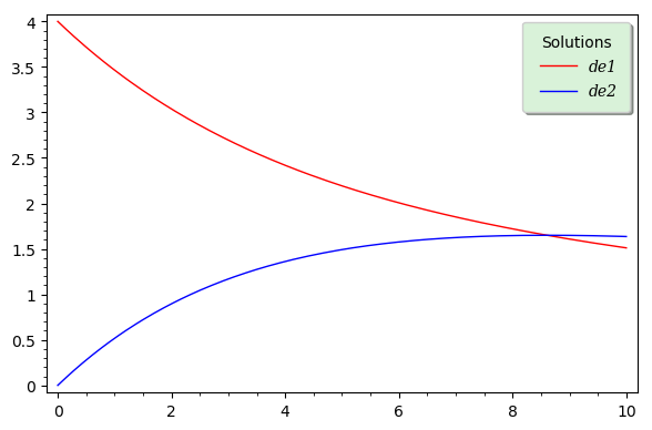
The code below completes your code, as well as that by @dsejas, adding a label to the plot. It also shows an alternative way of extracting the solutions $x(t)$ and $y(t)$ in order to define $f(t)$ and $g(t)$. Concerning the legend, I have deliberately used many customization options, just for the purpose of illustrating them. For a complete list of options, first evaluate the code, then type p.set_legend_options?.

t = var('t')
x = function('x')(t)
y = function('y')(t)
de1 = diff(x,t) == -3/20*x + 1/12*y
de2 = diff(y,t) == 3/20*x-3/20*y
sol = desolve_system([de1,de2],[x,y],ics=[0,4,0])

f(t) = x(t).subs(sol)
g(t) = y(t).subs(sol)

p  = plot(f, (t, 0, 10), color='red', legend_label="de1")
p += plot(g, (t, 0, 10), color='blue', legend_label="de2")
legend_op = dict(loc=1, handlelength=3, handletextpad=0.5, 
                 labelspacing=0.6, borderpad=0.8, title="Solutions",
                 back_color=(0.85,0.95,0.85), fancybox=True, 
                 font_family="serif", font_style="italic")
p.set_legend_options(**legend_op)
p.show(frame=True, axes=False)

This is the result:

image description

edit flag offensive delete link more

Your Answer

Please start posting anonymously - your entry will be published after you log in or create a new account.

Add Answer

Question Tools

1 follower

Stats

Asked: 2020-03-27 21:59:50 +0100

Seen: 719 times

Last updated: Mar 21 '21