Revision history [back]
| | 1 | initial version |
Hello, @PolarizedIce! If what you mean by "plot a differential equation" is "plot it's solution", your code is really close. You can do the following:
t = var('t')
x = function('x')(t)
y = function('y')(t)
de1 = diff(x,t) == -3/20*x + 1/12*y
de2 = diff(y,t) == 3/20*x-3/20*y
sol = desolve_system([de1,de2],[x,y],ics=[0,4,0])
f(t) = sol[0].rhs()
g(t) = sol[1].rhs()
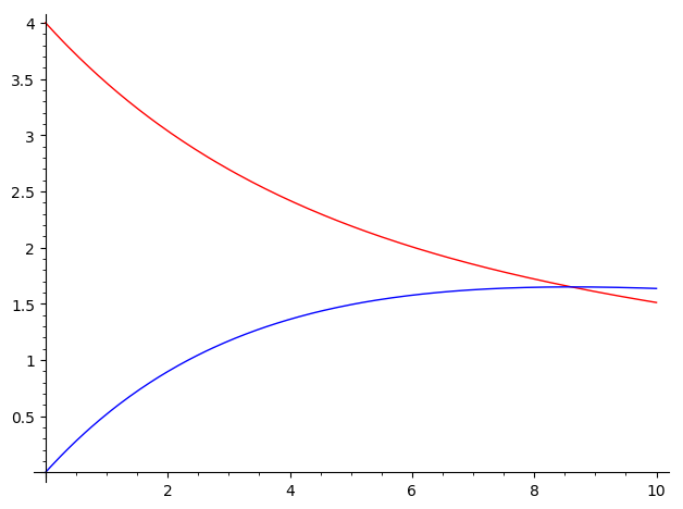
p = plot(f, (t, 0, 10), color='red')
p += plot(g, (t, 0, 10), color='blue')
p.show()
Here, I used the color option just to make clear which function is which. You can also plot both functions at the same time:
plot([f,g], (t,0,10))
As an alternative, in this particular case, you can also use the desolve_system_rk4 function:
t,x,y = var('t x y')
de1 = -3/20*x + 1/12*y
de2 = 3/20*x-3/20*y
sol = desolve_system_rk4([de1,de2], [x,y], ivar=t, ics=[4,0], end_points=10)
Notice that the differential equations must be of the form $\frac{dx}{dt}=F(x,t)$, so you use only the right-hand-side of your equations (see de1 and de2 in the previous code). Once you have specified the rhs of the equations, you specify the dependent variables, the independent variable, the initial condition (which is assumed to be valid for $t=0$, so you don't need to write the 0, as in the case of desolve_system), and finally, you introduce the final point of integration (I chose 10 in this case). You can also specify a step of integration with the step option (the default is step=0.1) . I must point out that desolve_system_rk4 solves the system numerically, as opposed to desolve_system, that solves symbolically.
In order to plot the numerical solution, you can do the following:
f = [(i,j) for i,j,k in sol]
g = [(i,k) for i,j,k in sol]
p = line(f, color='red')
p += line(g, color='blue')
p.show()
Whichever method you use, this should be the result:
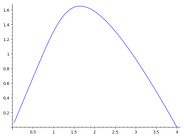
On the other hand, you can also plot the phase portrait. If you used the desolve_system, you should do
fp = [(f(t),g(t)) for t in srange(0,100,0.1)]
line(fp)
If you used desolve_system_rk4, you should do
fp = [(j,k) for i,j,k in sol]
line(fp)
Whatever method you used, the result should be like this:
I hope this helps!
| | 2 | No.2 Revision |
Hello, @PolarizedIce! If what you mean by "plot a differential equation" is "plot it's solution", your code is really close. You can do the following:
t = var('t')
x = function('x')(t)
y = function('y')(t)
de1 = diff(x,t) == -3/20*x + 1/12*y
de2 = diff(y,t) == 3/20*x-3/20*y
sol = desolve_system([de1,de2],[x,y],ics=[0,4,0])

f(t) = sol[0].rhs()
g(t) = sol[1].rhs()

p  = plot(f, (t, 0, 10), color='red')
p += plot(g, (t, 0, 10), color='blue')
p.show()
Here, I used the color option just to make clear which function is which. You can also plot both functions at the same time:
plot([f,g], (t,0,10))
As an alternative, in this particular case, you can also use the desolve_system_rk4 function:
t,x,y = var('t x y')
de1 = -3/20*x + 1/12*y
de2 = 3/20*x-3/20*y
sol = desolve_system_rk4([de1,de2], [x,y], ivar=t, ics=[4,0], ics=[0,4,0], end_points=10)
Notice that the differential equations must be of the form $\frac{dx}{dt}=F(x,t)$, so you use only the right-hand-side of your equations (see de1 and de2 in the previous code). Once you have specified the rhs of the equations, you specify the dependent variables, the independent variable, the initial condition (which is assumed to be valid for $t=0$, so you don't need to write the 0, as in the case of condition, and finally, you introduce the final point of integration (I chose 10 in this case). You can also specify a step of integration with the desolve_system), step option (the default is step=0.1) . I must point out that desolve_system_rk4 solves the system numerically, as opposed to desolve_system, that solves symbolically.
In order to plot the numerical solution, you can do the following:
f = [(i,j) for i,j,k in sol]
g = [(i,k) for i,j,k in sol]
p = line(f, color='red')
p += line(g, color='blue')
p.show()
Whichever method you use, this should be the result:
On the other hand, you can also plot the phase portrait. If you used the desolve_system, you should do
fp = [(f(t),g(t)) for t in srange(0,100,0.1)]
line(fp)
If you used desolve_system_rk4, you should do
fp = [(j,k) for i,j,k in sol]
line(fp)
Whatever method you used, the result should be like this:
I hope this helps!
| | 3 | No.3 Revision |
Hello, @PolarizedIce! If what you mean by "plot a differential equation" is "plot it's solution", your code is really close. You can do the following:
t = var('t')
x = function('x')(t)
y = function('y')(t)
de1 = diff(x,t) == -3/20*x + 1/12*y
de2 = diff(y,t) == 3/20*x-3/20*y
sol = desolve_system([de1,de2],[x,y],ics=[0,4,0])

f(t) = sol[0].rhs()
g(t) = sol[1].rhs()

p  = plot(f, (t, 0, 10), color='red')
p += plot(g, (t, 0, 10), color='blue')
p.show()
Here, I used the color option just to make clear which function is which. You can also plot both functions at the same time:
plot([f,g], (t,0,10))
As an alternative, in this particular case, you can also use the desolve_system_rk4 function:
t,x,y = var('t x y')
de1 = -3/20*x + 1/12*y
de2 = 3/20*x-3/20*y
sol = desolve_system_rk4([de1,de2], [x,y], ivar=t, ics=[0,4,0], end_points=10)
Notice that the differential equations must be of the form $\frac{dx}{dt}=F(x,t)$, so you use only the right-hand-side of your equations (see de1 and de2 in the previous code). Once you have specified the rhs of the equations, you specify the dependent variables, the independent variable, the initial condition, and finally, you introduce the final point of integration (I chose 10 in this case). You can also specify a step of integration with the step option (the default is step=0.1) . I must point out that desolve_system_rk4 solves the system numerically, as opposed to desolve_system, that solves symbolically.
In order to plot the numerical solution, you can do the following:
f = [(i,j) for i,j,k in sol]
g = [(i,k) for i,j,k in sol]
p = line(f, color='red')
p += line(g, color='blue')
p.show()
Whichever method you use, this should be the result:
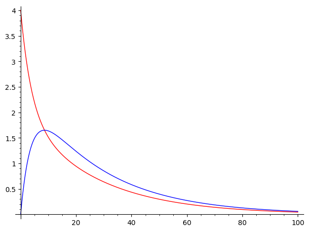
On the other hand, you can also plot the phase portrait. If you used the desolve_system, you should do
fp = [(f(t),g(t)) for t in srange(0,100,0.1)]
line(fp)
If you used desolve_system_rk4, you could change end_points=10 to end_points=100, in order to have a better output, and then you should do
fp = [(j,k) for i,j,k in sol]
line(fp)
Whatever method you used, the result should be like this:
I hope this helps!
| | 4 | No.4 Revision |
Hello, @PolarizedIce! If what you mean by "plot a differential equation" is "plot it's solution", your code is really close. You can do the following:
t = var('t')
x = function('x')(t)
y = function('y')(t)
de1 = diff(x,t) == -3/20*x + 1/12*y
de2 = diff(y,t) == 3/20*x-3/20*y
sol = desolve_system([de1,de2],[x,y],ics=[0,4,0])

f(t) = sol[0].rhs()
g(t) = sol[1].rhs()

p  = plot(f, (t, 0, 10), color='red')
p += plot(g, (t, 0, 10), color='blue')
p.show()
Here, I used the color option just to make clear which function is which. You can also plot both functions at the same time:
plot([f,g], (t,0,10))
As an alternative, in this particular case, you can also use the desolve_system_rk4 function:
t,x,y = var('t x y')
de1 = -3/20*x + 1/12*y
de2 = 3/20*x-3/20*y
sol = desolve_system_rk4([de1,de2], [x,y], ivar=t, ics=[0,4,0], end_points=10)
end_points=100)
Notice that the differential equations must be of the form $\frac{dx}{dt}=F(x,t)$, so you use only the right-hand-side of your equations (see de1 and de2 in the previous code). Once you have specified the rhs of the equations, you specify the dependent variables, the independent variable, the initial condition, and finally, you introduce the final point of integration (I chose 10 in this case). You can also specify a step of integration with the step option (the default is step=0.1) . I must point out that desolve_system_rk4 solves the system numerically, as opposed to desolve_system, that solves symbolically.
In order to plot the numerical solution, you can do the following:
f = [(i,j) for i,j,k in sol]
g = [(i,k) for i,j,k in sol]
p = line(f, color='red')
p += line(g, color='blue')
p.show()
Whichever method you use, this should be the result:
On the other hand, you can also plot the phase portrait. If you used the desolve_system, you should do
fp = [(f(t),g(t)) for t in srange(0,100,0.1)]
line(fp)
If you used desolve_system_rk4, you could change end_points=10 to end_points=100, in order to have a better output, and then you should do
fp = [(j,k) for i,j,k in sol]
line(fp)
Whatever method you used, the result should be like this:
I hope this helps!
| | 5 | No.5 Revision |
Hello, @PolarizedIce! If what you mean by "plot a differential equation" is "plot it's solution", your code is really close. You can do the following:
t = var('t')
x = function('x')(t)
y = function('y')(t)
de1 = diff(x,t) == -3/20*x + 1/12*y
de2 = diff(y,t) == 3/20*x-3/20*y
sol = desolve_system([de1,de2],[x,y],ics=[0,4,0])

f(t) = sol[0].rhs()
g(t) = sol[1].rhs()

p  = plot(f, (t, 0, 10), color='red')
p += plot(g, (t, 0, 10), color='blue')
p.show()
Here, I used the color option just to make clear which function is which. You can also plot both functions at the same time:
plot([f,g], (t,0,10))
As an alternative, in this particular case, you can also use the desolve_system_rk4 function:
t,x,y = var('t x y')
de1 = -3/20*x + 1/12*y
de2 = 3/20*x-3/20*y
sol = desolve_system_rk4([de1,de2], [x,y], ivar=t, ics=[0,4,0], end_points=100)
Notice that the differential equations must be of the form $\frac{dx}{dt}=F(x,t)$, so you use only the right-hand-side of your equations (see de1 and de2 in the previous code). Once you have specified the rhs of the equations, you specify the dependent variables, the independent variable, the initial condition, and finally, you introduce the final point of integration (I chose 10 in this case). You can also specify a step of integration with the step option (the default is step=0.1) . I must point out that desolve_system_rk4 solves the system numerically, as opposed to desolve_system, that solves symbolically.
In order to plot the numerical solution, you can do the following:
f = [(i,j) for i,j,k in sol]
g = [(i,k) for i,j,k in sol]
p = line(f, color='red')
p += line(g, color='blue')
p.show()
Whichever method you use, this should be the result:
On the other hand, you can also plot the phase portrait. If you used the desolve_system, you should do
fp = [(f(t),g(t)) for t in srange(0,100,0.1)]
line(fp)
If you used desolve_system_rk4, you could change then you should doend_points=10 to end_points=100, in order to have a better output, and
fp = [(j,k) for i,j,k in sol]
line(fp)
Whatever method you used, the result should be like this:
I hope this helps!
| | 6 | No.6 Revision |
Hello, @PolarizedIce! If what you mean by "plot a differential equation" is "plot it's solution", your code is really close. You can do the following:
t = var('t')
x = function('x')(t)
y = function('y')(t)
de1 = diff(x,t) == -3/20*x + 1/12*y
de2 = diff(y,t) == 3/20*x-3/20*y
sol = desolve_system([de1,de2],[x,y],ics=[0,4,0])

f(t) = sol[0].rhs()
g(t) = sol[1].rhs()

p  = plot(f, (t, 0, 10), 100), color='red')
p += plot(g, (t, 0, 10), 100), color='blue')
p.show()
Here, I used the color option just to make clear which function is which. You can also plot both functions at the same time:
plot([f,g], (t,0,10))
(t,0,100))
As an alternative, in this particular case, you can also use the desolve_system_rk4 function:
t,x,y = var('t x y')
de1 = -3/20*x + 1/12*y
de2 = 3/20*x-3/20*y
sol = desolve_system_rk4([de1,de2], [x,y], ivar=t, ics=[0,4,0], end_points=100)
Notice that the differential equations must be of the form $\frac{dx}{dt}=F(x,t)$, so you use only the right-hand-side of your equations (see de1 and de2 in the previous code). Once you have specified the rhs of the equations, you specify the dependent variables, the independent variable, the initial condition, and finally, you introduce the final point of integration (I chose 10 in this case). You can also specify a step of integration with the step option (the default is step=0.1) . I must point out that desolve_system_rk4 solves the system numerically, as opposed to desolve_system, that solves symbolically.
In order to plot the numerical solution, you can do the following:
f = [(i,j) for i,j,k in sol]
g = [(i,k) for i,j,k in sol]
p = line(f, color='red')
p += line(g, color='blue')
p.show()
Whichever method you use, this should be the result:
On the other hand, you can also plot the phase portrait. If you used the desolve_system, you should do
fp = [(f(t),g(t)) for t in srange(0,100,0.1)]
line(fp)
If you used desolve_system_rk4, then you should do
fp = [(j,k) for i,j,k in sol]
line(fp)
Whatever method you used, the result should be like this:
I hope this helps!
