Revision history [back]
| | 1 | initial version |

Although the syntax
region = implicit_plot3d(equation, range_x, range_y, range_z, region=restrictions)
region.show()
works well, I recommend to use this other approach:
region = implicit_plot3d(equation, range_x, range_y, range_z, region=restrictions)
region = region.add_condition(restrictions)
region.show()
Compare, for example, the output of
var("x,y,z")
region = implicit_plot3d(z==0, (x, -3, 3), (y, -3, 3), (z, -3, 3),
                         region=lambda x,y,z: y - 2*x<= 0 and 0<x and x<2 and 0<y and y<3)
region.show()
and
var("x,y,z")
region = implicit_plot3d(z==0, (x, -3, 3), (y, -3, 3), (z, -3, 3))
region = region.add_condition(lambda x,y,z: y - 2*x<= 0 and 0<x and x<2 and 0<y and y<3)
region.show()
Off course, adding the plot_points option, you can improve both pictures.
I conjecture that, given a bounded region $D\subset\mathbb{R}^2$ and a non-negative, integrable function $f:D\to\mathbb{R}$, you want to explain that $\iint_D f(x,y)\,dx\,dy$ is the volumen of the solid
This may explain why you want to plot $D$ in 3D space and why you ask in a comment how to get a solid. Consider, for example, that $D$ is the region you gave and that $f(x,y)=1+\sin^2(xy)$. In such a case, the solid $Q$ has six faces, which are portions of the graph of $f$ and the planes $x=2$, $y-2x=0$, $y=0$, $y=3$ and $z=0$. To keep things simple, you can plot each face with implicit_plot3d, adding the restrictions needed to get the exact portion that limits $Q$. The following code implements these ideas:
var("x,y,z")
range_x = (x, -0.5, 2.5)
range_y = (y, -0.5, 3.5)
range_z = (z, -0.5, 2.5)

f(x,y) = 1 + sin(x*y)^2

top = implicit_plot3d(f(x,y), range_x, range_y, range_z, color="green")
top = top.add_condition(lambda x,y,z: 0<=x<=2 and 0<=y<=3 and y-2*x<=0)

bottom = implicit_plot3d(z==0, range_x, range_y, range_z, color="brown")
bottom = bottom.add_condition(lambda x,y,z: 0<=x<=2 and 0<=y<=3 and y-2*x<=0)

front = implicit_plot3d(y==0, range_x, range_y, range_z, color="red")
front = front.add_condition(lambda x,y,z: 0<=x<=2 and y-2*x<=0 and 0<=z<=f(x,y))

back = implicit_plot3d(y==3, range_x, range_y, range_z, color="orange")
back = back.add_condition(lambda x,y,z: bool(0<=x<=2 and y-2*x<=0 and 0<=z<=f(x,y)))

left = implicit_plot3d(y-2*x==0, range_x, range_y, range_z, color="blue")
left = left.add_condition(lambda x,y,z: 0<=x<=2 and 0<=y<=3 and 0<=z<=f(x,y))

right = implicit_plot3d(x==2, range_x, range_y, range_z, color="cyan")
right = right.add_condition(lambda x,y,z: 0<=y<=3 and 0<=z<=f(x,y))

show(graph + bottom + front + back + left + right)
I offer several screenshots:
| | 2 | No.2 Revision |
Although the syntax
region = implicit_plot3d(equation, range_x, range_y, range_z, region=restrictions)
region.show()
works well, I recommend to use this other approach:
region = implicit_plot3d(equation, range_x, range_y, range_z, region=restrictions)
region = region.add_condition(restrictions)
region.show()
Compare, for example, the output of
var("x,y,z")
region = implicit_plot3d(z==0, (x, -3, 3), (y, -3, 3), (z, -3, 3),
                         region=lambda x,y,z: y - 2*x<= 0 and 0<x and x<2 and 0<y and y<3)
region.show()
and
var("x,y,z")
region = implicit_plot3d(z==0, (x, -3, 3), (y, -3, 3), (z, -3, 3))
region = region.add_condition(lambda x,y,z: y - 2*x<= 0 and 0<x and x<2 and 0<y and y<3)
region.show()
Off course, adding the plot_points option, you can improve both pictures.
I conjecture that, given a bounded region $D\subset\mathbb{R}^2$ and a non-negative, integrable function $f:D\to\mathbb{R}$, you want to explain that $\iint_D f(x,y)\,dx\,dy$ is the volumen of the solid
This may explain why you want to plot $D$ in 3D space and why you ask in a comment how to get a solid. Consider, for example, that $D$ is the region you gave and that $f(x,y)=1+\sin^2(xy)$. In such a case, the solid $Q$ has six faces, which are portions of the graph of $f$ and the planes $x=2$, $y-2x=0$, $y=0$, $y=3$ and $z=0$. To keep things simple, you can plot each face with implicit_plot3d, adding the restrictions needed to get the exact portion that limits $Q$. The following code implements these ideas:
var("x,y,z")
range_x = (x, -0.5, 2.5)
range_y = (y, -0.5, 3.5)
range_z = (z, -0.5, 2.5)

f(x,y) = 1 + sin(x*y)^2

top = implicit_plot3d(f(x,y), implicit_plot3d(z==f(x,y), range_x, range_y, range_z, color="green")
top = top.add_condition(lambda x,y,z: 0<=x<=2 and 0<=y<=3 and y-2*x<=0)

bottom = implicit_plot3d(z==0, range_x, range_y, range_z, color="brown")
bottom = bottom.add_condition(lambda x,y,z: 0<=x<=2 and 0<=y<=3 and y-2*x<=0)

front = implicit_plot3d(y==0, range_x, range_y, range_z, color="red")
front = front.add_condition(lambda x,y,z: 0<=x<=2 and y-2*x<=0 and 0<=z<=f(x,y))

back = implicit_plot3d(y==3, range_x, range_y, range_z, color="orange")
back = back.add_condition(lambda x,y,z: bool(0<=x<=2 and y-2*x<=0 and 0<=z<=f(x,y)))

left = implicit_plot3d(y-2*x==0, range_x, range_y, range_z, color="blue")
left = left.add_condition(lambda x,y,z: 0<=x<=2 and 0<=y<=3 and 0<=z<=f(x,y))

right = implicit_plot3d(x==2, range_x, range_y, range_z, color="cyan")
right = right.add_condition(lambda x,y,z: 0<=y<=3 and 0<=z<=f(x,y))

show(graph + bottom + front + back + left + right)
I offer several screenshots:
| | 3 | No.3 Revision |
Although the syntax
region = implicit_plot3d(equation, range_x, range_y, range_z, region=restrictions)
region.show()
works well, I recommend to use this other approach:
region = implicit_plot3d(equation, range_x, range_y, range_z, region=restrictions)
region = region.add_condition(restrictions)
region.show()
Compare, for example, the output of
var("x,y,z")
region = implicit_plot3d(z==0, (x, -3, 3), (y, -3, 3), (z, -3, 3),
                         region=lambda x,y,z: y - 2*x<= 0 and 0<x and x<2 and 0<y and y<3)
region.show()
and
var("x,y,z")
region = implicit_plot3d(z==0, (x, -3, 3), (y, -3, 3), (z, -3, 3))
region = region.add_condition(lambda x,y,z: y - 2*x<= 0 and 0<x and x<2 and 0<y and y<3)
region.show()
Off course, adding the plot_points option, you can improve both pictures.
I conjecture that, given a bounded region $D\subset\mathbb{R}^2$ and a non-negative, integrable function $f:D\to\mathbb{R}$, you want to explain that $\iint_D f(x,y)\,dx\,dy$ is the volumen of the solid
This may explain why you want to plot $D$ in 3D space and why you ask in a comment how to get a solid. Consider, for example, that $D$ is the region you gave and that $f(x,y)=1+\sin^2(xy)$. In such a case, the solid $Q$ has six faces, which are portions of the graph of $f$ and the planes $x=2$, $y-2x=0$, $y=0$, $y=3$ and $z=0$. To keep things simple, you can plot each face with implicit_plot3d, adding the restrictions needed to get the exact portion that limits $Q$. However, the top surface looks better if obtained with `plot3d`. The following code implements these ideas:
var("x,y,z")
range_x = (x, -0.5, 2.5)
range_y = (y, -0.5, 3.5)
range_z = (z, -0.5, 2.5)

f(x,y) = 1 + sin(x*y)^2

top = implicit_plot3d(z==f(x,y), range_x, range_y, range_z, color="green")
plot3d(f(x,y), range_x, range_y, color="green", plot_points=100)
top = top.add_condition(lambda x,y,z: 0<=x<=2 and 0<=y<=3 and y-2*x<=0)

bottom = implicit_plot3d(z==0, range_x, range_y, range_z, color="brown")
bottom = bottom.add_condition(lambda x,y,z: 0<=x<=2 and 0<=y<=3 and y-2*x<=0)

front = implicit_plot3d(y==0, range_x, range_y, range_z, color="red")
front = front.add_condition(lambda x,y,z: 0<=x<=2 and y-2*x<=0 and 0<=z<=f(x,y))

back = implicit_plot3d(y==3, range_x, range_y, range_z, color="orange")
back = back.add_condition(lambda x,y,z: bool(0<=x<=2 and y-2*x<=0 and 0<=z<=f(x,y)))

left = implicit_plot3d(y-2*x==0, range_x, range_y, range_z, color="blue")
left = left.add_condition(lambda x,y,z: 0<=x<=2 and 0<=y<=3 and 0<=z<=f(x,y))

right = implicit_plot3d(x==2, range_x, range_y, range_z, color="cyan")
right = right.add_condition(lambda x,y,z: 0<=y<=3 and 0<=z<=f(x,y))

show(graph show(top + bottom + front + back + left + right)
I offer several screenshots:
| | 4 | No.4 Revision |
Although the syntax
region = implicit_plot3d(equation, range_x, range_y, range_z, region=restrictions)
region.show()
works well, I recommend to use this other approach:
region = implicit_plot3d(equation, range_x, range_y, range_z, region=restrictions)
region = region.add_condition(restrictions)
region.show()
Compare, for example, the output of
var("x,y,z")
region = implicit_plot3d(z==0, (x, -3, 3), (y, -3, 3), (z, -3, 3),
                         region=lambda x,y,z: y - 2*x<= 0 and 0<x and x<2 and 0<y and y<3)
region.show()
and
var("x,y,z")
region = implicit_plot3d(z==0, (x, -3, 3), (y, -3, 3), (z, -3, 3))
region = region.add_condition(lambda x,y,z: y - 2*x<= 0 and 0<x and x<2 and 0<y and y<3)
region.show()
Off course, adding the plot_points option, you can improve both pictures.
I conjecture that, given a bounded region $D\subset\mathbb{R}^2$ and a non-negative, integrable function $f:D\to\mathbb{R}$, you want to explain that $\iint_D f(x,y)\,dx\,dy$ is the volumen of the solid
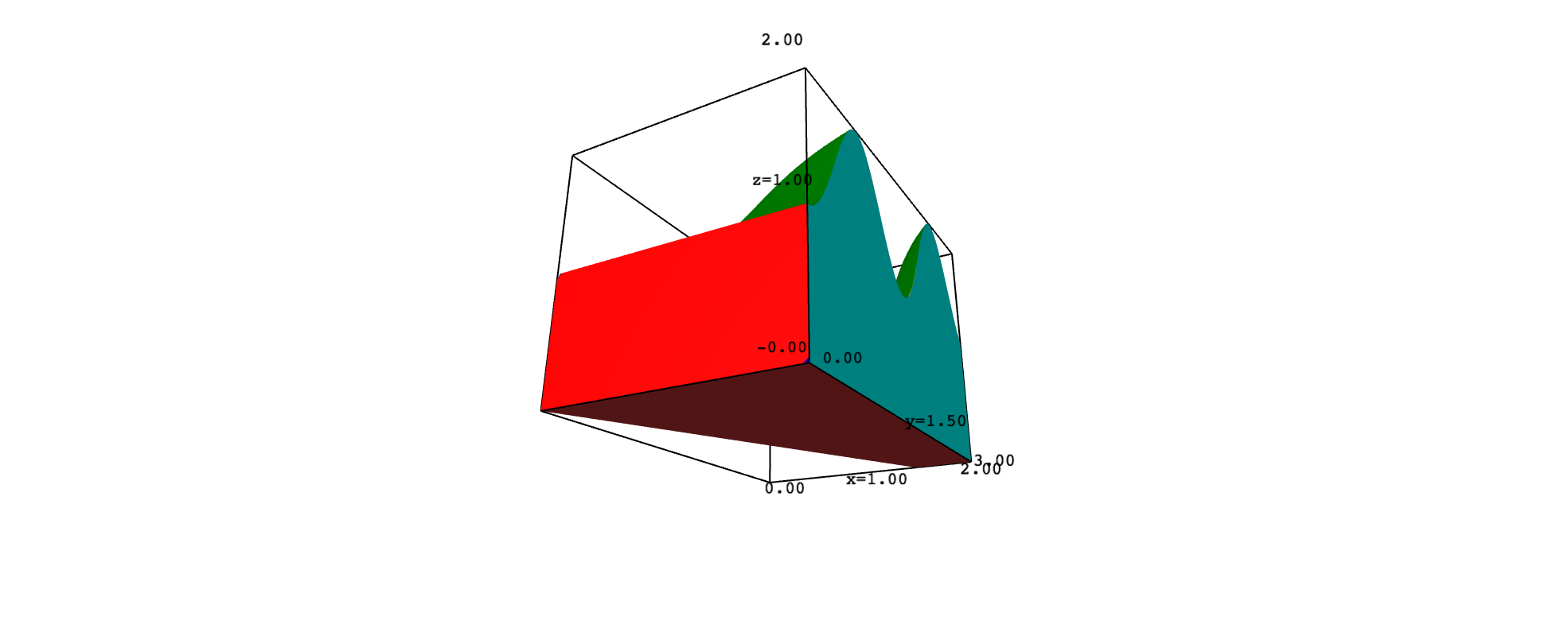
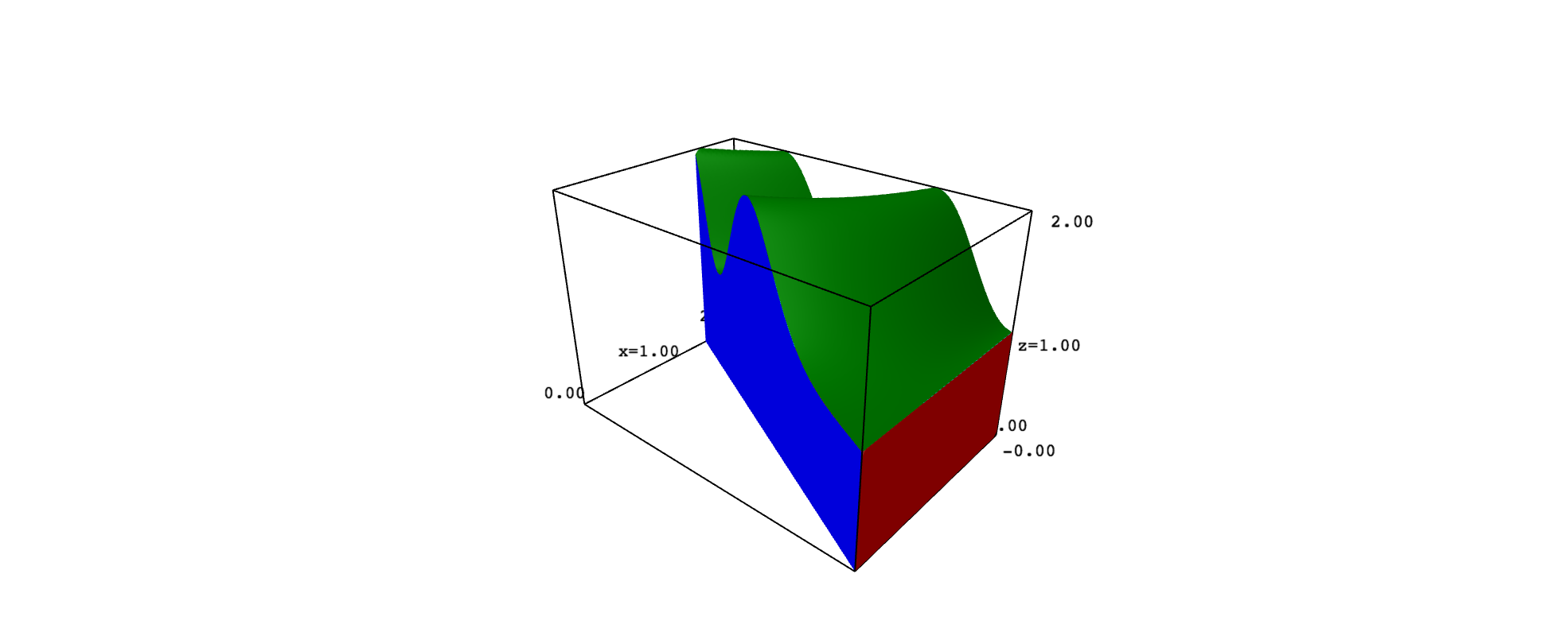
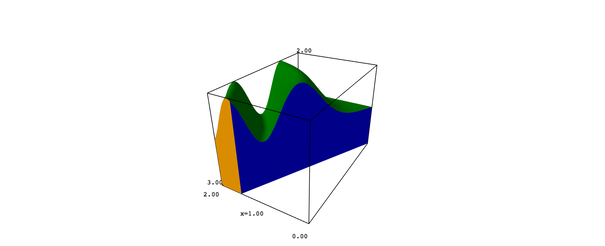
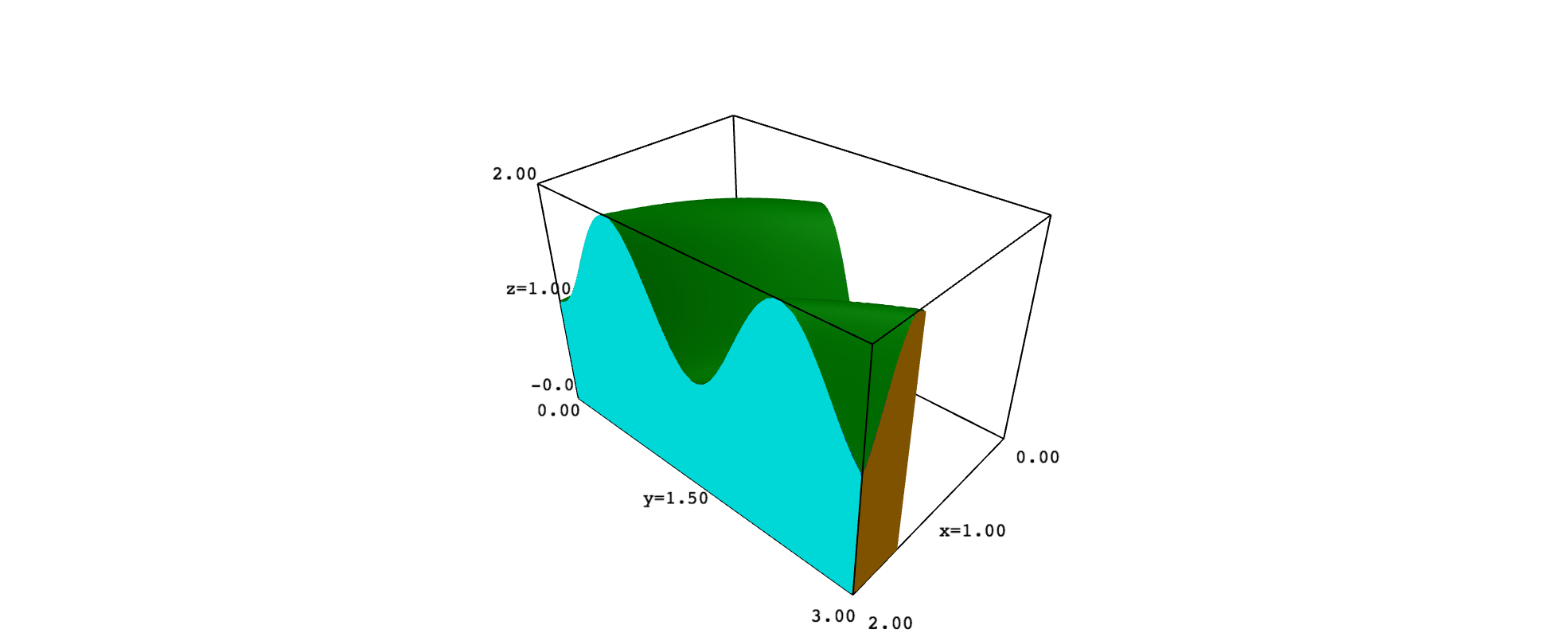
This may explain why you want to plot $D$ in 3D space and why you ask in a comment how to get a solid. Consider, for example, that $D$ is the region you gave and that $f(x,y)=1+\sin^2(xy)$. In such a case, the solid $Q$ has six faces, which are portions of the graph of $f$ and the planes $x=2$, $y-2x=0$, $y=0$, $y=3$ and $z=0$. To keep things simple, you can plot each face with implicit_plot3d, adding the restrictions needed to get the exact portion that limits $Q$. However, the top surface looks better if obtained with `plot3d`. plot3d. The following code implements these ideas:
var("x,y,z")
range_x = (x, -0.5, 2.5)
range_y = (y, -0.5, 3.5)
range_z = (z, -0.5, 2.5)

f(x,y) = 1 + sin(x*y)^2

top = plot3d(f(x,y), range_x, range_y, color="green", plot_points=100)
top = top.add_condition(lambda x,y,z: 0<=x<=2 and 0<=y<=3 and y-2*x<=0)

bottom = implicit_plot3d(z==0, range_x, range_y, range_z, color="brown")
bottom = bottom.add_condition(lambda x,y,z: 0<=x<=2 and 0<=y<=3 and y-2*x<=0)

front = implicit_plot3d(y==0, range_x, range_y, range_z, color="red")
front = front.add_condition(lambda x,y,z: 0<=x<=2 and y-2*x<=0 and 0<=z<=f(x,y))

back = implicit_plot3d(y==3, range_x, range_y, range_z, color="orange")
back = back.add_condition(lambda x,y,z: bool(0<=x<=2 and y-2*x<=0 and 0<=z<=f(x,y)))

left = implicit_plot3d(y-2*x==0, range_x, range_y, range_z, color="blue")
left = left.add_condition(lambda x,y,z: 0<=x<=2 and 0<=y<=3 and 0<=z<=f(x,y))

right = implicit_plot3d(x==2, range_x, range_y, range_z, color="cyan")
right = right.add_condition(lambda x,y,z: 0<=y<=3 and 0<=z<=f(x,y))

show(top + bottom + front + back + left + right)
I offer several screenshots:
