[ Note : you should try to avoit fixing the arguments a=of a symbolic function... ]
sage: f = function('f')
sage: de = diff(f(x),x,2) + 4*diff(f(x),x) + 5*f(x) == 15*cos(4*x)
sage: PM = desolve(de, f(x), ivar=x, ics=(0,0,0))
sage: PM
15/377*(11*cos(x) - 42*sin(x))*e^(-2*x) - 165/377*cos(4*x) + 240/377*sin(4*x)
The expressions of the shape $a\cos(u)+ b\sin(u)$ can indeed be expressed as $c\cos(u+d)$, but that is irrelevant to your question. More relevant is to consider your function as a polynomial of the dampening function $e^{-2x}$
sage: PM.subs(e^(-2*x)==E2X).coefficients(E2X)
[[-165/377*cos(4*x) + 240/377*sin(4*x), 0],
 [165/377*cos(x) - 630/377*sin(x), 1]]
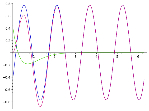
This decomposition allows to decompose your function as the sum of a "steady" and a "dampened" functions :
sage: fs, fd = ((u[0]*E2X^u[1]).subs(E2X==e^(-2*x)).function(x) for u in PM.subs(e^(-2*x)==E2X).coefficients(E2X))
sage: fs
x |--> -165/377*cos(4*x) + 240/377*sin(4*x)
sage: fd
x |--> 15/377*(11*cos(x) - 42*sin(x))*e^(-2*x)
The plot is therefore trivial :
sage: plot((fs, fd, fs+fd),(x, 0, 2*pi))
Launched png viewer for Graphics object consisting of 3 graphics primitives
HTH,
EDIT : If you are interested in the trigonometric expressions manipulation, here's how to transform your expressions :
sage: a, b, c, d = var("a, b, c, d")
The expected form :
sage: Eq=a*cos(x) + b*sin(x) == c*cos(d + x) ; Eq
a*cos(x) + b*sin(x) == c*cos(d + x)
This relation must be true for any value of $\sin x$ and $cos x$ ; it is therefore implicitly a system of (polynomial equations in $\sin x$ and $cos x$, which we can get explicitly :
sage: Sys=[(Eq.lhs()-Eq.rhs()).trig_expand().coefficient(u(x),1) for u in (sin, cos)] ; Sys
[c*sin(d) + b, -c*cos(d) + a]
Neither Maxima nor Giac or Fricas can directly solve this system, which we will solve manually. Get a first expression of $c$ :
sage: Sc=Sys[1].solve(c)[0] ; Sc
c == a/cos(d)
which we use to get (a function of) $d$ :
sage: St=(((Sys[0].subs(Sc)==0)-b)/a).trig_reduce() ; St
tan(d) == -b/a
We can now get $c^2$ :
sage: Sc2=(Sc.solve(cos(d))[0]^2).subs(cos(d)^2==1/(1+tan(d)^2)).subs(St).solve(c^2) ; Sc2
[c^2 == a^2 + b^2]
Note that we have to manually introduce $\tan d$. We can now get our candidate solutions :
sage: Sol=[[St.solve(d)[0], u] for u in Sc2[0].solve(c)] ; Sol
[[d == -arctan(b/a), c == -sqrt(a^2 + b^2)],
 [d == -arctan(b/a), c == sqrt(a^2 + b^2)]]
Since we have used a solution of $c^2$ to get a solution for $c$, we may have introduced a spurious solution. Indeed, the first solution doesn't check :
sage: bool(Eq.subs(Sol[0]).simplify_full().canonicalize_radical())
False
but the second one does :
sage: bool(Eq.subs(Sol[1]).simplify_full().canonicalize_radical())
True
Note that Mathematica
also needs a manual explicitation of the implicit system,
expresses its results in an awkward form, not easily simplifiable :
i. e. :
 sage: mathematica.Solve([(Eq.lhs()-Eq.rhs()).trig_expand().coefficient(u(x),1)==0 for u in (sin, cos)], [c, d])
{{c -> -(a^2/Sqrt[a^2 + b^2]) - b^2/Sqrt[a^2 + b^2],
  d -> ConditionalExpression[ArcTan[-(a/Sqrt[a^2 + b^2]),
      b/Sqrt[a^2 + b^2]] + 2*Pi*C[1], Element[C[1], Integers]]},
 {c -> a^2/Sqrt[a^2 + b^2] + b^2/Sqrt[a^2 + b^2],
  d -> ConditionalExpression[ArcTan[a/Sqrt[a^2 + b^2],
      -(b/Sqrt[a^2 + b^2])] + 2*Pi*C[1], Element[C[1], Integers]]}}

sage: mathematica.Simplify(mathematica.Solve([(Eq.lhs()-Eq.rhs()).trig_expand().coefficient(u(x),1)==0 for u in (sin, cos)], [c, d]))
{{c -> -Sqrt[a^2 + b^2], d -> ConditionalExpression[
    ArcTan[-(a/Sqrt[a^2 + b^2]), b/Sqrt[a^2 + b^2]] + 2*Pi*C[1],
    Element[C[1], Integers]]}, {c -> Sqrt[a^2 + b^2],
  d -> ConditionalExpression[ArcTan[a/Sqrt[a^2 + b^2],
      -(b/Sqrt[a^2 + b^2])] + 2*Pi*C[1], Element[C[1], Integers]]}}

sage: mathematica.FullSimplify(mathematica.Solve([(Eq.lhs()-Eq.rhs()).trig_expand().coefficient(u(x),1)==0 for u in (sin, cos)], [c, d]))
{{c -> -Sqrt[a^2 + b^2], d -> ConditionalExpression[
    2*Pi*C[1] - I*Log[-((a - I*b)/Sqrt[a^2 + b^2])],
    Element[C[1], Integers]]}, {c -> Sqrt[a^2 + b^2],
  d -> ConditionalExpression[2*Pi*C[1] - I*Log[(a - I*b)/Sqrt[a^2 + b^2]],
    Element[C[1], Integers]]}}
Sympy can solve the same system, but its solution is ... disputable... :
sage: SS = solve(Sys, [c, d], algorithm="sympy") ; SS
[{c: -(a^2 + b^2 - sqrt(a^2 + b^2)*a)/(a - sqrt(a^2 + b^2)),
  d: 2*arctan((a - sqrt(a^2 + b^2))/b)},
 {c: -(a^2 + b^2 + sqrt(a^2 + b^2)*a)/(a + sqrt(a^2 + b^2)),
  d: 2*arctan((a + sqrt(a^2 + b^2))/b)}]
One can note that :
sage: ((SS[0][c].numerator()*(a^2 + b^2 + sqrt(a^2 + b^2)*a)).expand()/((SS[0][c].denominator()*(a^2 + b^2 + sqrt(a^2 + b^2)*a)).expand())).factor()
sqrt(a^2 + b^2)
sage: ((SS[1][c].numerator()*(sqrt(a^2 + b^2)*a-(a^2 + b^2 ))).expand()/((SS[1][c].denominator()*(sqrt(a^2 + b^2)*a-(a^2 + b^2 ))).expand())).simplify_full()
-sqrt(a^2 + b^2)
and
sage: tan(SS[0][d]).trig_expand().expand().canonicalize_radical()
-b/a
sage: tan(SS[1][d]).trig_expand().expand().canonicalize_radical()
-b/a
The solutions given by Sympy are therefore identical to those manually obtained ; the same limitations apply. However, their properties are way less obvious, and their transformation to "easier" forms quite unintuitive...
EDIT 2: Pulling it all together :
f = function('f')
de = diff(f(x),x,2) + 4*diff(f(x),x) + 5*f(x) == 15*cos(4*x)
PM = desolve(de, f(x), ivar=x, ics=(0,0,0))
PM0, PM1 = ((u[0]*(e^(-2*x))^u[1]) for u in PM.coefficients(e^(-2*x)))
var('a, b, c, d')
Eq0 = PM0 - a*cos(4*x + b).trig_expand()
S0 = solve([Eq0.coefficient(u(4*x), 1) for u in (sin, cos)],[a, b],
         algorithm = "sympy")
check0 = all([Eq0.subs(s).simplify_full() == 0 for s in S0])
fs = (a*cos(4*x + b)).subs(S0[0]).function(x)
Eq1 = (PM1/e^(-2*x) - c*cos(x+d).trig_expand())
S1=solve([Eq1.coefficient(u(x), 1) for u in (sin, cos)], (c, d), algorithm="sympy")
check1 = all([Eq1.subs(s).simplify_full() == 0 for s in S1])
fd = ((c*cos(x + d)).subs(S1[0])*e^(-2*x)).function(x)
ft = fs + fd
The result can be seen as :
plot((fs, fd, ft), (0, 2*pi), legend_label=["fs", "fd", "ft"], axes=False, frame=True)
HTH,
