Weird resulting values with an exponential regression

asked 2016-09-01 16:50:40 +0200

Romuald_314
115 ●6 ●9 ●17

updated 2016-09-01 16:56:35 +0200

John Palmieri

8551 ●19 ●71 ●186 http://www.math.washin...

I have this model:

var('a,b')
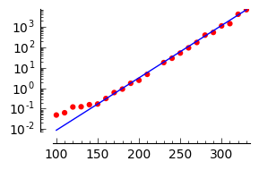
R = [[100, 0.0489], [110, 0.0633], [120, 0.1213],[130, 0.1244], [140, 0.1569], [150, 0.1693], [160, 0.3154], [170, 0.6146], [180, 0.9118], [190, 01.7478], [200, 2.4523], [210, 4.7945], [230, 17.9766], [240, 29.3237], [250, 52.4374], [260, 94.6463], [270, 173.3447], [280, 396.0443], [290, 538.6976], [300, 1118.9984], [310, 1442.3694], [320, 4151.9089], [330, 6940.7322]]

model(x) = a*exp(b*x)

find_fit(R,model)

(which is the results of factorization time of an algorithm for people interested)

But I get weird values, obviously not in accordance with the points, when plotting all this. I was extremely surprised. That's what I get:

[a=(2.3863359829×10^−15),b=1.0000000003]

Then I had the idea to try to get a formula with LibreOffice calc, just to have something to compare (I wasn't about to do this work on libreoffice initially), the result is different, but still so weird. In both cases, if I apply the formula given, it returns unthinkable values (very high).

Seems to be a problem with these values, no? Impossible to compute? Does sb have a solution? Thank you.

edit retag flag offensive close merge delete

Comments

This seems to be the same problem in Scipy as http://ask.sagemath.org/question/2643...

kcrisman ( 2016-09-01 17:55:43 +0200 )edit

Really? That's annoying... By the way the SageMathCell gives the same thing. I think it must be the programs, not powerful enough (or the algorithms) to work with exponentials, big amount of data... that's delicate as a function. I've experienced similar problems in python (not with math and regressions): it was supposed to work fine and there were errors no one could understand. Weird problems, in short...

Romuald_314 ( 2016-09-01 19:48:14 +0200 )edit

The result of FindFit[] in Mathematica 10 is {a -> 0., b -> 1.}

paulmasson ( 2016-09-01 21:30:04 +0200 )edit

That doesn't really help -- and th'at's also false.

Romuald_314 ( 2016-09-02 20:43:19 +0200 )edit

I think paulmasson's point was that it means this is the kind of data that standard regression models don't do well with in general...

kcrisman ( 2016-09-02 21:45:06 +0200 )edit

see more comments

3 Answers

Sort by » oldest newest most voted

answered 2017-09-23 11:59:10 +0200

Emmanuel Charpentier
7057 ●6 ●46 ●137

Being a) a statistician and b) lazy to the extreme, I tend to use well-validated tools that I know... R being in Sage, my minimal-effort solution is :

sage: Data=[[100, 0.0489], [110, 0.0633], [120, 0.1213],[130, 0.1244], [140, 0.1569], [150, 0.1693], [160, 0.3154], [170
....: , 0.6146], [180, 0.9118], [190, 01.7478], [200, 2.4523], [210, 4.7945], [230, 17.9766], [240, 29.3237], [250, 52.4
....: 374], [260, 94.6463], [270, 173.3447], [280, 396.0443], [290, 538.6976], [300, 1118.9984], [310, 1442.3694], [320,
....:  4151.9089], [330, 6940.7322]]
sage: RData=r.data_frame(X=[t[0] for t in Data], Y=[t[1] for t in Data])
sage: RModel=r.as_formula("log(Y)~X")
sage: r.summary(r.lm(RModel, data=RData))

Call:
lm(formula = sage103, data = sage166)

Residuals:
     Min       1Q   Median       3Q      Max
-0.55634 -0.34349 -0.09318  0.25851  0.86680

Coefficients:
             Estimate Std. Error t value Pr(>|t|)
(Intercept) -9.214846   0.283884  -32.46   <2e-16 ***
X            0.053301   0.001255   42.45   <2e-16 ***
---
Signif. codes:  0 ‘***’ 0.001 ‘**’ 0.01 ‘*’ 0.05 ‘.’ 0.1 ‘ ’ 1

Residual standard error: 0.4257 on 21 degrees of freedom
Multiple R-squared:  0.9885,    Adjusted R-squared:  0.9879
F-statistic:  1802 on 1 and 21 DF,  p-value: < 2.2e-16

This is in good concordance with paulmason' results (I would have been quite surprised if this was not the case...), and gives Romuald_314 the $R^2$ he asked for.

edit flag offensive delete link

add a comment

answered 2016-09-01 21:55:24 +0200

paulmasson
1580 ●1 ●24 ●45 http://analyticphysics...

Rather than trying to fit the data directly, how about fitting its logarithm:

var('a,b')
R = [[100, 0.0489], [110, 0.0633], [120, 0.1213],[130, 0.1244], [140, 0.1569], [150, 0.1693], [160, 0.3154], [170, 0.6146], [180, 0.9118], [190, 01.7478], [200, 2.4523], [210, 4.7945], [230, 17.9766], [240, 29.3237], [250, 52.4374], [260, 94.6463], [270, 173.3447], [280, 396.0443], [290, 538.6976], [300, 1118.9984], [310, 1442.3694], [320, 4151.9089], [330, 6940.7322]]

logR = []
for r in R:
    logR.append( [ r[0], log(r[1]) ] )

model(x) = a*x + b

fit = find_fit(logR, model)
print fit

p = scatter_plot(R)
p += plot( exp(a*x+b).subs(fit[0],fit[1]), (x,0,340) )
show(p)

The result of fitting the logarithm is

[a == 0.053300682674800925, b == -9.214845890267727]

which of course needs to be exponentiated to compare to the original data.

Here's a live example showing plots of the original data and the fit.

edit flag offensive delete link

Comments

Thank you paulmasson, seems to work fine now ! Now I can have a line such as

ln(y) = a*x+b

Romuald_314 ( 2016-09-02 20:46:23 +0200 )edit

Just one question about regressions: can we have the coefficient R^2 ??

Romuald_314 ( 2016-09-02 21:17:46 +0200 )edit

That coefficient is not exposed by SageMath. You'll have to calculate it yourself.

paulmasson ( 2016-09-02 21:42:38 +0200 )edit

Alternately, you could use R fitting tools - if you are really interested in that kind of stuff you should probably be using pandas or R in any case. But a lot of times theoretical bounds end up not being so close to the actual performance for "small" values that today's computers can access :)

kcrisman ( 2016-09-02 21:43:53 +0200 )edit

I see. Actually, I tried to calculate that coefficient before, without any conclusive outcome. I'll have to be looking for a formula.

Romuald_314 ( 2016-09-03 08:22:13 +0200 )edit

add a comment

answered 2017-09-19 14:45:13 +0200

This post is a wiki. Anyone with karma >750 is welcome to improve it.

var('b')

R = [[100, 0.0489], [110, 0.0633], [120, 0.1213],[130, 0.1244], [140, 0.1569], [150, 0.1693], [160, 0.3154], [170, 0.6146], [180, 0.9118], [190, 01.7478], [200, 2.4523], [210, 4.7945], [230, 17.9766], [240, 29.3237], [250, 52.4374], [260, 94.6463], [270, 173.3447], [280, 396.0443], [290, 538.6976], [300, 1118.9984], [310, 1442.3694], [320, 4151.9089], [330, 6940.7322]]

Ro=150

mo=0.1693

model(x) = mo*exp(b*(x-Ro))

fit=find_fit(R,model,solution_dict=True)

plot(model.subs(fit),(x,100,330))+points(R,size=20,color='red',figsize=3)

plot