Revision history [back]

As suggested above, a graphical representation gives an easy intuition :

plot([(I^x).abs(), (I^x).maxima_methods().arg()], (x, -3, 3), legend_label=["Modulus", "Argument"])

To understand the result, try :

sage: var("a, b")
(a, b)
sage: E0=log(a^b)==log(a^b).log_expand() ; E0
log(a^b) == b*log(a)
sage: E1 =E0.subs([a==I, b==x]) ; E1
log(I^x) == 1/2*I*pi*x
sage: E2 = E1.operator()(*map(exp, E1.operands())) ; E2
I^x == e^(1/2*I*pi*x)

The latter may be easier to grasp in a different form :

sage: E2.rhs().demoivre(force=True)
cos(1/2*pi*x) + I*sin(1/2*pi*x)

Exercise for the (advanced) reader : try and understand :

complex_plot(I^x, (-1, 1), (-1, 1))

![Complex plot of $e^iz}$

Hint : look up the definitions of exp and trig functions for complexes...

HTH,

As suggested above, a graphical representation gives an easy intuition :

plot([(I^x).abs(), (I^x).maxima_methods().arg()], (x, -3, 3), legend_label=["Modulus", "Argument"])

To understand the result, try :

sage: var("a, b")
(a, b)
sage: E0=log(a^b)==log(a^b).log_expand() ; E0
log(a^b) == b*log(a)
sage: E1 =E0.subs([a==I, b==x]) ; E1
log(I^x) == 1/2*I*pi*x
sage: E2 = E1.operator()(*map(exp, E1.operands())) ; E2
I^x == e^(1/2*I*pi*x)

The latter may be easier to grasp in a different form :

sage: E2.rhs().demoivre(force=True)
cos(1/2*pi*x) + I*sin(1/2*pi*x)

Exercise for the (advanced) reader : try and understand :

complex_plot(I^x, (-1, 1), (-1, 1))

![Complex plot of $e^iz}$

Hint : look up the definitions of exp and trig functions for complexes...

HTH,

As suggested above, a graphical representation gives an easy intuition :

plot([(I^x).abs(), (I^x).maxima_methods().arg()], (x, -3, 3), legend_label=["Modulus", "Argument"])

To understand the result, try :

sage: var("a, b")
(a, b)
sage: E0=log(a^b)==log(a^b).log_expand() ; E0
log(a^b) == b*log(a)
sage: E1 =E0.subs([a==I, b==x]) ; E1
log(I^x) == 1/2*I*pi*x
sage: E2 = E1.operator()(*map(exp, E1.operands())) ; E2
I^x == e^(1/2*I*pi*x)

The latter may be easier to grasp in a different form :

sage: E2.rhs().demoivre(force=True)
cos(1/2*pi*x) + I*sin(1/2*pi*x)

Exercise for the (advanced) reader : try and understand :

complex_plot(I^x, (-1, 1), (-1, 1))
(-3, 3), (-3, 3))

![Complex plot of $e^iz}$

Hint : look up the definitions of exp and trig functions for complexes...

EDIT : The complex_plot is displayed in the editor, but does not appear in the finalized answer. Try it on your machine or Sagecell

HTH,

As suggested above, a graphical representation gives an easy intuition :

plot([(I^x).abs(), (I^x).maxima_methods().arg()], (x, -3, 3), legend_label=["Modulus", "Argument"])

To understand the result, try :

sage: var("a, b")
(a, b)
sage: E0=log(a^b)==log(a^b).log_expand() ; E0
log(a^b) == b*log(a)
sage: E1 =E0.subs([a==I, b==x]) ; E1
log(I^x) == 1/2*I*pi*x
sage: E2 = E1.operator()(*map(exp, E1.operands())) ; E2
I^x == e^(1/2*I*pi*x)

The latter may be easier to grasp in a different form :

sage: E2.rhs().demoivre(force=True)
cos(1/2*pi*x) + I*sin(1/2*pi*x)

Exercise for the (advanced) reader : try and understand :

complex_plot(I^x, (-3, 3), (-3, 3))

![Complex plot of $e^iz}$

Hint : look up the definitions of exp and trig functions for complexes...

EDIT : The complex_plot is displayed in the editor, but does not appear in the finalized answer. Try it on your machine or Sagecell

HTH,

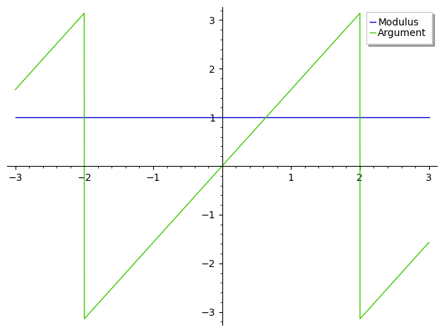
As suggested above, a graphical representation gives an easy intuition :

plot([(I^x).abs(), (I^x).maxima_methods().arg()], (x, -3, 3), legend_label=["Modulus", "Argument"])

To understand the result, try :

sage: var("a, b")
(a, b)
sage: E0=log(a^b)==log(a^b).log_expand() ; E0
log(a^b) == b*log(a)
sage: E1 =E0.subs([a==I, b==x]) ; E1
log(I^x) == 1/2*I*pi*x
sage: E2 = E1.operator()(*map(exp, E1.operands())) ; E2
I^x == e^(1/2*I*pi*x)

The latter may be easier to grasp in a different form :

sage: E2.rhs().demoivre(force=True)
cos(1/2*pi*x) + I*sin(1/2*pi*x)

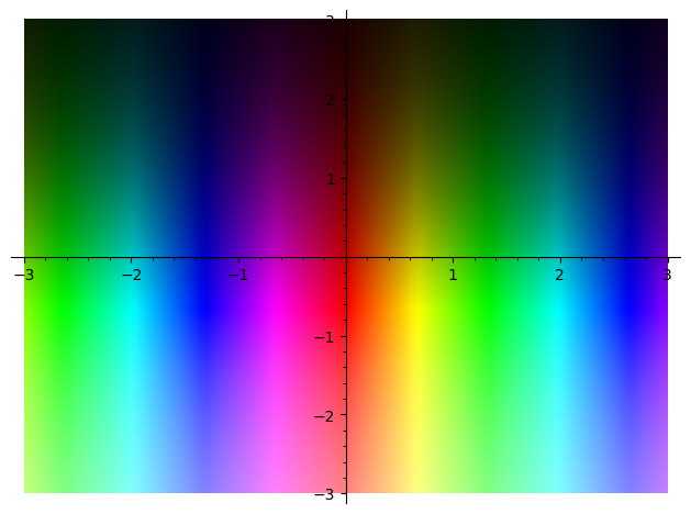
Exercise for the (advanced) reader : try and understand :

complex_plot(I^x, (-3, 3), (-3, 3))

Hint : look up the definitions of exp and trig functions for complexes...

EDIT : The complex_plot is displayed in the editor, but does not appear in the finalized answer. Try it on your machine or Sagecell

HTH,