Revision history [back]
| | 1 | initial version |
Not a fullanswer, but a (high-school level) hint, which, combined with FredericCs big fat one, should give you a solution :
Define the curve as a parametric callable symbolic expression :
t  = SR.var("t")
C(t) = vector([cos(t), sin(t), t/2])
Tangeant :
T(t) = vector(map(lambda u:u.diff(t), C(t)))
# Its norm is time independant...
Tn = T(t).norm().simplify_full()
Normal (= acceleration)
N(t) = vector(map(lambda u:u.function(t).diff(t,2), C(t)))
# Again, time-independent norm :
Nn = N(t).norm().simplify_full()
Binormal :
B(t) = T(t).cross_product(N(t))
# Ditto...
Bn = B(t).norm().simplify_full()
A vector of points where we want to plot Frenet's trihedron
tPts = srange(-pi, 11*pi/10, pi/5)
3D plot of the curve itself :
P1 = parametric_plot3d(C, (-pi, pi), color="black")
Plot the (normed) tangeants :
P2 = sum(map(lambda u:line((C(u),C(u)+T(u)/Tn), color="blue", arrow_head=True),
             tPts))
The normals :
P3 = sum(map(lambda u:line((C(u),C(u)+N(u)/Nn), color="red", arrow_head=True),
             tPts))
The binormals :
P4 = sum(map(lambda u:line((C(u),C(u)+B(u)/Bn), color="green", arrow_head=True),
             tPts))
Now, perusing parametric_plot3d? will show you that this function can plot surfaces having two parameters. This should be more than enough for your goal...
Note that Sage's abilities in differential geometry my give you some radical different solutions. Left as an exercise for the (advanced) reader.
HTH,
| | 2 | No.2 Revision |
Not a fullanswer, (yet) a full answer (but see edit below if you are really stuck), but a (high-school level) hint, which, combined with FredericCs big fat one, should give you a solution :
Define the curve as a parametric callable symbolic expression :
t  = SR.var("t")
C(t) = vector([cos(t), sin(t), t/2])
Tangeant :
T(t) = vector(map(lambda u:u.diff(t), C(t)))
# Its norm is time independant...
Tn = T(t).norm().simplify_full()
Normal (= acceleration)
N(t) = vector(map(lambda u:u.function(t).diff(t,2), C(t)))
# Again, time-independent norm :
Nn = N(t).norm().simplify_full()
Binormal :
B(t) = T(t).cross_product(N(t))
# Ditto...
Bn = B(t).norm().simplify_full()
A vector of points where we want to plot Frenet's trihedron
tPts = srange(-pi, 11*pi/10, pi/5)
3D plot of the curve itself :
P1 = parametric_plot3d(C, (-pi, pi), color="black")
Plot the (normed) tangeants :
P2 = sum(map(lambda u:line((C(u),C(u)+T(u)/Tn), color="blue", arrow_head=True),
             tPts))
The normals :
P3 = sum(map(lambda u:line((C(u),C(u)+N(u)/Nn), color="red", arrow_head=True),
             tPts))
The binormals :
P4 = sum(map(lambda u:line((C(u),C(u)+B(u)/Bn), color="green", arrow_head=True),
             tPts))
Now, perusing parametric_plot3d? will show you that this function can plot surfaces having two parameters. This should be more than enough for your goal...
EDIT : Do not read this before doing an honest attempt at finding the solution yourself ; otherwise, you'd lose the benefit of the homework).
This result can be used to get the desired plot. Let's define a description of the normal section of the tube (here a circle of radius r) : the vector (N(t)/Nn, B(t)/Bn) is an orthonormal basis of the plane normal to C(t). Therefore, this description is :
# Radius of a circular-section tube
var("r")
# Parametric desription of the normal section of the tube
Ts(t,theta)=N(t)/Nn*r*cos(theta)+B(t)/Bn*r*sin(theta)
and the description of any point of the tube is :
# A point of the tube
Tu(t,theta)=C(t)+Ts(t, theta)
which can be plotted (along with its center curve) by :
P1 + parametric_plot3d(Tu.subs(r==1/3), (-pi, pi), (0, 2*pi), opacity=0.5)
which should give you something along the lines of :
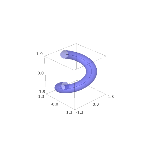
Note that Sage's abilities in differential geometry my may give you some radical radically different solutions. Left as an exercise for the (advanced) reader.
Bonus points : extrapolate to this...
HTH,
| | 3 | No.3 Revision |
Not (yet) a full answer (but see edit below if you are really stuck), but a (high-school level) hint, which, combined with FredericCs big fat one, should give you a solution :
Define the curve as a parametric callable symbolic expression :
t  = SR.var("t")
C(t) = vector([cos(t), sin(t), t/2])
Tangeant :
T(t) = vector(map(lambda u:u.diff(t), C(t)))
# Its norm is time independant...
Tn = T(t).norm().simplify_full()
Normal (= acceleration)
N(t) = vector(map(lambda u:u.function(t).diff(t,2), C(t)))
# Again, time-independent norm :
Nn = N(t).norm().simplify_full()
Binormal :
B(t) = T(t).cross_product(N(t))
# Ditto...
Bn = B(t).norm().simplify_full()
A vector of points where we want to plot Frenet's trihedron
tPts = srange(-pi, 11*pi/10, pi/5)
3D plot of the curve itself :
P1 = parametric_plot3d(C, (-pi, pi), color="black")
Plot the (normed) tangeants :
P2 = sum(map(lambda u:line((C(u),C(u)+T(u)/Tn), color="blue", arrow_head=True),
             tPts))
The normals :
P3 = sum(map(lambda u:line((C(u),C(u)+N(u)/Nn), color="red", arrow_head=True),
             tPts))
The binormals :
P4 = sum(map(lambda u:line((C(u),C(u)+B(u)/Bn), color="green", arrow_head=True),
             tPts))
Now, perusing parametric_plot3d? will show you that this function can plot surfaces having two parameters. This should be more than enough for your goal...
EDIT : Do not read this before doing an honest attempt at finding the solution yourself ; otherwise, you'd lose the benefit of the homework).
This result can be used to get the desired plot. Let's define a description of the normal section of the tube (here a circle of radius r) : the vector (N(t)/Nn, B(t)/Bn) is an orthonormal basis of the plane normal to C(t). Therefore, this description is :
# Radius of a circular-section tube
var("r")
# Parametric desription of the normal section of the tube
Ts(t,theta)=N(t)/Nn*r*cos(theta)+B(t)/Bn*r*sin(theta)
and the description of any point of the tube is :
# A point of the tube
Tu(t,theta)=C(t)+Ts(t, theta)
which can be plotted (along with its center curve) by :
P1 + parametric_plot3d(Tu.subs(r==1/3), (-pi, pi), (0, 2*pi), opacity=0.5)
which should give you something along the lines of :
Note that Sage's abilities in differential geometry may give you some radically different solutions. Left as an exercise for the (advanced) reader.
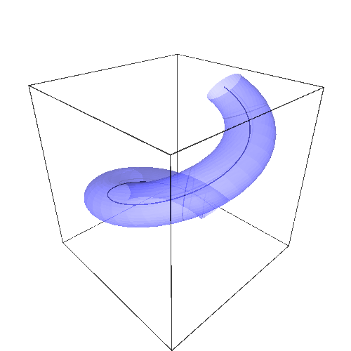
Bonus points : extrapolate to this...... ;-)
HTH,
