Revision history [back]
| | 1 | initial version |

Are you working on dessins d'enfants ?
Here is a simple idea for an approximate plot
sage: x = polygen(QQ, 'x')
sage: f = 1/729*(2*x**2-3*x+9)**3*(x+1)
sage: N = 50
sage: sum(point2d(root) for k in range(N+1) for root in (f - k / N).complex_roots())
| | 2 | No.2 Revision |
Are you working on dessins d'enfants ?d'enfants?
Here is a simple idea for an approximate plotplot.
sage: x = polygen(QQ, 'x')
sage: f = 1/729*(2*x**2-3*x+9)**3*(x+1)
sage: N = 50
sage: sum(point2d(root) point2d(root for k in range(N+1) for root in (f - k / N).complex_roots())
The function pre01 below builds on this idea.
It gives a good idea of the desired plot and runs very fast.
def pre01(f, n=50, **opt):
    r"""
    Return the preimage of the unit interval under this rational function.

    INPUT:

    - ``f`` -- a rational function

    - ``n`` -- optional (default: 50) -- roughly how many points
      in the unit interval [0, 1] to use for preparing the plot

    Roughly a third or the points are inverse powers of two,
    roughly a third are one minus inverse powers of two,
    and roughly a third are linearly spaced along the interval.

    EXAMPLES::

        sage: x = polygen(QQ, 'x')
        sage: f = 1/729 * (2 * x**2 - 3 * x + 9)**3 * (x + 1)
        sage: pre01(f, n=50, color='teal').show(figsize=5)

        sage: z = polygen(QQ, 'z')
        sage: num = -(z^4-6*z^3+12*z^2-8*z)*(z-1)^3*(z-3)
        sage: den = (2*z-3)*(z-2)^3*z
        sage: pre01(num/den, n=50, color='steelblue').show(figsize=7)

        sage: Qz.<z> = QQ[]
        sage: cc = [81, -432, 972, -1200, 886, -400, 108, -16, 1]
        sage: num = -Qz(cc)*(z-2)^6*(z-4)*z
        sage: den = (6*z^4-48*z^3+140*z^2-176*z+81)*(z-1)^4*(z-3)^4
        sage: pre01(num/den, n=50, color='firebrick').show(figsize=7)
    """
    nn = n // 3 + 2
    num, den = f.numerator(), f.denominator()
    tt = [0] + [ZZ(2)**-k for k in (0 .. nn)]
    tt.extend([1 - t for t in tt[3:]])
    tt.extend(QQ((k, nn)) for k in (1 .. nn - 1))
    zz = (root for t in set(tt) for root in (num - t*den).complex_roots())
    cols = {'color': 'teal', 'axes_color': 'grey',
            'axes_label_color': 'grey', 'tick_label_color': 'grey'}
    op = {'size': 4, 'color': 'teal', 'zorder': 3, 'aspect_ratio': 1}
    for k, v in opt.items():
        if 'color' in k:
            cols[k] = v
        else
            op[k] = v
    G = point2d(zz, color=cols['color'] **op)
    G.axes_color(cols['axes_color'])
    G.axes_label_color(cols['axes_label_color'])
    G.tick_label_color(cols['tick_label_color'])
    return G
Three examples of usage.
Our quick example from above:
x = polygen(QQ, 'x')
f = 1/729 * (2 * x**2 - 3 * x + 9)**3 * (x + 1)
p = pre01(f, n=50, color='teal')
p.show(figsize=5)
The first example in the question:
z = polygen(QQ, 'z')
num = -(z^4-6*z^3+12*z^2-8*z)*(z-1)^3*(z-3)
den = (2*z-3)*(z-2)^3*z
p = pre01(num/den, n=50, color='steelblue')
p.show(figsize=5)
The second example in the question:
z = polygen(QQ, 'z')
num = -(z^8-16*z^7+108*z^6-400*z^5+886*z^4-1200*z^3+972*z^2-432*z+81)*(z-2)^6*(z-4)*z
den = (6*z^4-48*z^3+140*z^2-176*z+81)*(z-1)^4*(z-3)^4
p = pre01(num/den, n=50, color='firebrick')
p.show(figsize=5)
Each of those three examples runs in under a second.
| | 3 | No.3 Revision |
Are you working on dessins d'enfants?
Here is a simple idea for an approximate plot.
sage: x = polygen(QQ, 'x')
sage: f = 1/729*(2*x**2-3*x+9)**3*(x+1)
sage: N = 50
sage: point2d(root for k in range(N+1) for root in (f - k / N).complex_roots())
The function pre01 below builds on this idea.
idea.
It gives a good idea of the desired plot and runs very fast.
def pre01(f, n=50, **opt):
    r"""
    Return the preimage of the unit interval under this rational function.

    INPUT:

    - ``f`` -- a rational function

    - ``n`` -- optional (default: 50) -- roughly how many points
      in the unit interval [0, 1] to use for preparing the plot

    Roughly a third or the points are inverse powers of two,
    roughly a third are one minus inverse powers of two,
    and roughly a third are linearly spaced along the interval.

    EXAMPLES::

        sage: x = polygen(QQ, 'x')
        sage: f = 1/729 * (2 * x**2 - 3 * x + 9)**3 * (x + 1)
        sage: pre01(f, n=50, color='teal').show(figsize=5)

        sage: z = polygen(QQ, 'z')
        sage: num = -(z^4-6*z^3+12*z^2-8*z)*(z-1)^3*(z-3)
        sage: den = (2*z-3)*(z-2)^3*z
        sage: pre01(num/den, n=50, color='steelblue').show(figsize=7)
color='steelblue').show(figsize=5)

        sage: Qz.<z> = QQ[]
        sage: cc = [81, -432, 972, -1200, 886, -400, 108, -16, 1]
        sage: num = -Qz(cc)*(z-2)^6*(z-4)*z
        sage: den = (6*z^4-48*z^3+140*z^2-176*z+81)*(z-1)^4*(z-3)^4
        sage: pre01(num/den, n=50, color='firebrick').show(figsize=7)
color='firebrick').show(figsize=5)
    """
    nn = n // 3 + 2
    num, den = f.numerator(), f.denominator()
    tt = [0] + [ZZ(2)**-k for k in (0 .. nn)]
    tt.extend([1 - t for t in tt[3:]])
    tt.extend(QQ((k, nn)) for k in (1 .. nn - 1))
    zz = (root for t in set(tt) for root in (num - t*den).complex_roots())
    cols = {'color': 'teal', 'axes_color': 'grey',
            'axes_label_color': 'grey', 'tick_label_color': 'grey'}
    op = {'size': 4, 'color': 'teal', 'zorder': 3, 'aspect_ratio': 1}
    for k, v in opt.items():
        if 'color' in k:
            cols[k] = v
        else
else:
            op[k] = v
    G = point2d(zz, color=cols['color'] **op)
    G.axes_color(cols['axes_color'])
    G.axes_label_color(cols['axes_label_color'])
    G.tick_label_color(cols['tick_label_color'])
    return G
Three examples of usage.using this function follow.
Our quick example from above:
x = polygen(QQ, 'x')
f = 1/729 * (2 * x**2 - 3 * x + 9)**3 * (x + 1)
p = pre01(f, n=50, color='teal')
p.show(figsize=5)
The first example in the question:
z = polygen(QQ, 'z')
num = -(z^4-6*z^3+12*z^2-8*z)*(z-1)^3*(z-3)
den = (2*z-3)*(z-2)^3*z
p = pre01(num/den, n=50, color='steelblue')
p.show(figsize=5)
The second example in the question:
z = polygen(QQ, 'z')
num = -(z^8-16*z^7+108*z^6-400*z^5+886*z^4-1200*z^3+972*z^2-432*z+81)*(z-2)^6*(z-4)*z
den = (6*z^4-48*z^3+140*z^2-176*z+81)*(z-1)^4*(z-3)^4
p = pre01(num/den, n=50, color='firebrick')
p.show(figsize=5)
Each of those three examples runs in under a second.
| | 4 | No.4 Revision |
Are you working on dessins d'enfants?
Here is a simple idea for an approximate plot.
sage: x = polygen(QQ, 'x')
sage: f = 1/729*(2*x**2-3*x+9)**3*(x+1)
sage: N = 50
sage: point2d(root for k in range(N+1) for root in (f - k / N).complex_roots())
The function pre01 below builds on this idea.
It gives a good idea of the desired plot and runs fast.
def pre01(f, n=50, **opt):
    r"""
    Return the preimage of the unit interval under this rational function.

    INPUT:

    - ``f`` -- a rational function

    - ``n`` -- optional (default: 50) -- roughly how many points
      in the unit interval [0, 1] to use for preparing the plot

    Roughly a third or the points are inverse powers of two,
    roughly a third are one minus inverse powers of two,
    and roughly a third are linearly spaced along the interval.

    EXAMPLES::

        sage: x = polygen(QQ, 'x')
        sage: f = 1/729 * (2 * x**2 - 3 * x + 9)**3 * (x + 1)
        sage: pre01(f, n=50, color='teal').show(figsize=5)

        sage: z = polygen(QQ, 'z')
        sage: num = -(z^4-6*z^3+12*z^2-8*z)*(z-1)^3*(z-3)
        sage: den = (2*z-3)*(z-2)^3*z
        sage: pre01(num/den, n=50, color='steelblue').show(figsize=5)

        sage: Qz.<z> = QQ[]
        sage: cc = [81, -432, 972, -1200, 886, -400, 108, -16, 1]
        sage: num = -Qz(cc)*(z-2)^6*(z-4)*z
        sage: den = (6*z^4-48*z^3+140*z^2-176*z+81)*(z-1)^4*(z-3)^4
        sage: pre01(num/den, n=50, color='firebrick').show(figsize=5)
    """
    nn = n // 3 + 2
    num, den = f.numerator(), f.denominator()
    tt = [0] + [ZZ(2)**-k for k in (0 .. nn)]
    tt.extend([1 - t for t in tt[3:]])
    tt.extend(QQ((k, nn)) for k in (1 .. nn - 1))
    zz = (root for t in set(tt) for root in (num - t*den).complex_roots())
    cols = {'color': 'teal', 'axes_color': 'grey',
            'axes_label_color': 'grey', 'tick_label_color': 'grey'}
    op = {'size': 4, 'color': 'teal', 'zorder': 3, 'aspect_ratio': 1}
    for k, v in opt.items():
        if 'color' in k:
            cols[k] = v
        else:
            op[k] = v
    G = point2d(zz, color=cols['color'] color=cols['color'], **op)
    G.axes_color(cols['axes_color'])
    G.axes_label_color(cols['axes_label_color'])
    G.tick_label_color(cols['tick_label_color'])
    return G
Three examples of using this function follow.
Our quick example from above:
x = polygen(QQ, 'x')
f = 1/729 * (2 * x**2 - 3 * x + 9)**3 * (x + 1)
p = pre01(f, n=50, color='teal')
p.show(figsize=5)
The first example in the question:
z = polygen(QQ, 'z')
num = -(z^4-6*z^3+12*z^2-8*z)*(z-1)^3*(z-3)
den = (2*z-3)*(z-2)^3*z
p = pre01(num/den, n=50, color='steelblue')
p.show(figsize=5)
The second example in the question:
z = polygen(QQ, 'z')
num = -(z^8-16*z^7+108*z^6-400*z^5+886*z^4-1200*z^3+972*z^2-432*z+81)*(z-2)^6*(z-4)*z
den = (6*z^4-48*z^3+140*z^2-176*z+81)*(z-1)^4*(z-3)^4
p = pre01(num/den, n=50, color='firebrick')
p.show(figsize=5)
Each of those three examples runs in under a second.
| | 5 | No.5 Revision |
Are you working on dessins d'enfants?
Here is a simple idea for an approximate plot.
sage: x = polygen(QQ, 'x')
sage: f = 1/729*(2*x**2-3*x+9)**3*(x+1)
sage: N = 50
sage: point2d(root for k in range(N+1) for root in (f - k / N).complex_roots())
The function pre01 below builds on this idea.
It gives a good idea of the desired plot and runs fast.
def pre01(f, n=50, style='dots', **opt):
    r"""
    Return the preimage of the unit interval under this rational function.

    INPUT:

    - ``f`` -- a rational function

    - ``n`` -- optional (default: 50) -- roughly how many points
      in the unit interval [0, 1] to use for preparing the plot

    Roughly a third or the points are inverse powers of two,
    roughly a third are one minus inverse powers of two,
    and roughly a third are linearly spaced along the interval.

    EXAMPLES::

        sage: x = polygen(QQ, 'x')
        sage: f = 1/729 * (2 * x**2 - 3 * x + 9)**3 * (x + 1)
        sage: pre01(f, n=50, color='teal').show(figsize=5)
style='dots', color='firebrick').show(figsize=5)
        sage: pre01(f, n=50, style='line', color='firebrick').show(figsize=5)

        sage: z = polygen(QQ, 'z')
        sage: num = -(z^4-6*z^3+12*z^2-8*z)*(z-1)^3*(z-3)
        sage: den = (2*z-3)*(z-2)^3*z
        sage: pre01(num/den, g = num/den
        sage: pre01(g, n=50, color='steelblue').show(figsize=5)
style='dots', color='firebrick').show(figsize=5)
        sage: pre01(g, n=50, style='line', color='firebrick').show(figsize=5)

        sage: Qz.<z> = QQ[]
        sage: cc = [81, -432, 972, -1200, 886, -400, 108, -16, 1]
        sage: num = -Qz(cc)*(z-2)^6*(z-4)*z
        sage: den = (6*z^4-48*z^3+140*z^2-176*z+81)*(z-1)^4*(z-3)^4
        sage: pre01(num/den, h = num/den
        sage: pre01(h, n=50, style='dots', color='firebrick').show(figsize=5)
        sage: pre01(h, n=50, style='line', color='firebrick').show(figsize=5)
    """
    nn = n // 3 + 2
    num, den = f.numerator(), f.denominator()
    tt = [0] + [ZZ(2)**-k for k in (0 .. nn)]
    tt.extend([1 - t for t in tt[3:]])
    tt.extend(QQ((k, nn)) for k in (1 .. nn - 1))
    zz = (root for t in set(tt) for root in (num - t*den).complex_roots())
tt = sorted(set(tt))
    cols = {'color': 'teal', 'axes': True, 'axes_color': 'grey',
            'axes_label_color': 'grey', 'tick_label_color': 'grey'}
    op = {'size': dop = {'aspect_ratio': 1, 'size': 4, 'color': 'teal', 'zorder': 3, 'aspect_ratio': 1}
10}
    lop = {'aspect_ratio': 1, 'edge_thickness': 2}
    for k, v in opt.items():
        if 'color' in k or 'axis' in k or 'axes' in k or 'tick' in k:
            cols[k] = v
        elif k == 'size':
            dop[k] = v
        elif k == 'edge_thickness':
            lop[k] = v
        else:
            op[k] dop[k] = lop[k] = v
    if style == 'dots':
        zz = (root for t in set(tt) for root in (num - t*den).complex_roots())
        G = point2d(zz, color=cols['color'], **op)
**dop)
    elif style == 'line':
        tzz = {t: (num - t*den).complex_roots() for t in tt}
        D = Graph()
        for k, t in enumerate(tt[1:-1], start=1):
            s, u = tt[k-1], tt[k+1]
            szz, uzz = tzz[s], tzz[u]
            for z in tzz[t]:
                zs = min((abs(z - w), w) for w in szz)[1]
                D.add_edge(z, zs, k-1)
                zu = min((abs(z - w), w) for w in uzz)[1]
                D.add_edge(z, zu, k)
        D.set_pos({z: (z.real(), z.imag()) for z in D})
        ecol = {cols['color']: D.edges()}
        G = D.plot(vertex_labels=False, vertex_size=0, edge_colors=ecol, **lop)
    else:
        raise ValueError(f"style should be 'dots' or 'line', got :'{style}'")
    G.axes(cols['axes'])
    G.axes_color(cols['axes_color'])
    G.axes_label_color(cols['axes_label_color'])
    G.tick_label_color(cols['tick_label_color'])
    return G
Three examples of using this function follow.
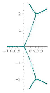
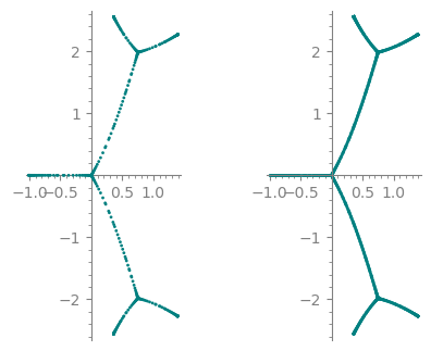
Our quick Quick starting example from above:of this answer:
x = polygen(QQ, 'x')
f = 1/729 * (2 * x**2 - 3 * x + 9)**3 * (x + 1)
p a_dots = pre01(f, n=50, style='dots, color='teal')
p.show(figsize=5)
a_line = pre01(f, n=50, style='line', color='teal')
a_dots_lines = graphics_array([a_dots, a_line], ncols=2)
a_dots_lines.show(figsize=5)
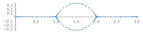
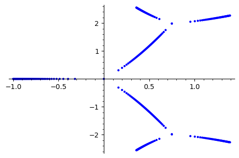
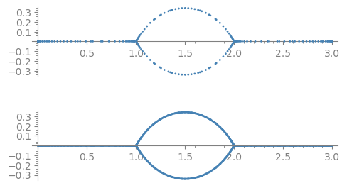
The first First example in the question:
z = polygen(QQ, 'z')
num = -(z^4-6*z^3+12*z^2-8*z)*(z-1)^3*(z-3)
den = (2*z-3)*(z-2)^3*z
p b_dots = pre01(num/den, n=50, style='dots', color='steelblue')
p.show(figsize=5)
b_line = pre01(num/den, n=50, style='line', color='steelblue')
b_dots_lines = graphics_array([b_dots, b_line], ncols=1)
b_dots_lines.show(figsize=5)
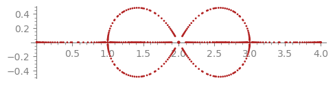
The second Second example in the question:
z = polygen(QQ, 'z')
num = -(z^8-16*z^7+108*z^6-400*z^5+886*z^4-1200*z^3+972*z^2-432*z+81)*(z-2)^6*(z-4)*z
den = (6*z^4-48*z^3+140*z^2-176*z+81)*(z-1)^4*(z-3)^4
p c_dots = pre01(num/den, n=50, style='dots', color='firebrick')
p.show(figsize=5)
c_line = pre01(num/den, n=50, style='line', color='firebrick')
c_dots_lines = graphics_array([c_dots, c_line], ncols=1)
c_dots_lines.show(figsize=5)
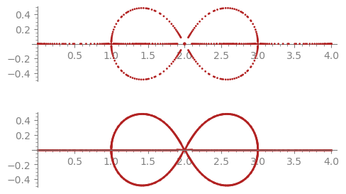
Each of those three examples runs in under a second.second per plot style.
| | 6 | No.6 Revision |
Are you working on dessins d'enfants?
Here is a simple idea for an approximate plot.
sage: x = polygen(QQ, 'x')
sage: f = 1/729*(2*x**2-3*x+9)**3*(x+1)
sage: N = 50
sage: point2d(root for k in range(N+1) for root in (f - k / N).complex_roots())
The function pre01 below builds on this idea.
It gives a good idea of the desired plot and runs fast.
def pre01(f, n=50, style='dots', **opt):
    r"""
    Return the preimage of the unit interval under this rational function.

    INPUT:

    - ``f`` -- a rational function

    - ``n`` -- optional (default: 50) -- roughly how many points
      in the unit interval [0, 1] to use for preparing the plot

    Roughly a third or the points are inverse powers of two,
    roughly a third are one minus inverse powers of two,
    and roughly a third are linearly spaced along the interval.

    EXAMPLES::

        sage: x = polygen(QQ, 'x')
        sage: f = 1/729 * (2 * x**2 - 3 * x + 9)**3 * (x + 1)
        sage: pre01(f, n=50, style='dots', color='firebrick').show(figsize=5)
        sage: pre01(f, n=50, style='line', color='firebrick').show(figsize=5)

        sage: z = polygen(QQ, 'z')
        sage: num = -(z^4-6*z^3+12*z^2-8*z)*(z-1)^3*(z-3)
        sage: den = (2*z-3)*(z-2)^3*z
        sage: g = num/den
        sage: pre01(g, n=50, style='dots', color='firebrick').show(figsize=5)
        sage: pre01(g, n=50, style='line', color='firebrick').show(figsize=5)

        sage: Qz.<z> = QQ[]
        sage: cc = [81, -432, 972, -1200, 886, -400, 108, -16, 1]
        sage: num = -Qz(cc)*(z-2)^6*(z-4)*z
        sage: den = (6*z^4-48*z^3+140*z^2-176*z+81)*(z-1)^4*(z-3)^4
        sage: h = num/den
        sage: pre01(h, n=50, style='dots', color='firebrick').show(figsize=5)
        sage: pre01(h, n=50, style='line', color='firebrick').show(figsize=5)
    """
    nn = n // 3 + 2
    num, den = f.numerator(), f.denominator()
    tt = [0] + [ZZ(2)**-k for k in (0 .. nn)]
    tt.extend([1 - t for t in tt[3:]])
    tt.extend(QQ((k, nn)) for k in (1 .. nn - 1))
    tt = sorted(set(tt))
    cols = {'color': 'teal', 'axes': True, 'axes_color': 'grey',
            'axes_label_color': 'grey', 'tick_label_color': 'grey'}
    dop = {'aspect_ratio': 1, 'size': 4, 'zorder': 10}
    lop = {'aspect_ratio': 1, 'edge_thickness': 2}
    for k, v in opt.items():
        if 'color' in k or 'axis' in k or 'axes' in k or 'tick' in k:
            cols[k] = v
        elif k == 'size':
            dop[k] = v
        elif k == 'edge_thickness':
            lop[k] = v
        else:
            dop[k] = lop[k] = v
    if style == 'dots':
        zz = (root for t in set(tt) for root in (num - t*den).complex_roots())
        G = point2d(zz, color=cols['color'], **dop)
    elif style == 'line':
        tzz = {t: (num - t*den).complex_roots() for t in tt}
        D = Graph()
        for k, t in enumerate(tt[1:-1], start=1):
            s, u = tt[k-1], tt[k+1]
            szz, uzz = tzz[s], tzz[u]
            for z in tzz[t]:
                zs = min((abs(z - w), w) for w in szz)[1]
                D.add_edge(z, zs, k-1)
                zu = min((abs(z - w), w) for w in uzz)[1]
                D.add_edge(z, zu, k)
        D.set_pos({z: (z.real(), z.imag()) for z in D})
        ecol = {cols['color']: D.edges()}
        G = D.plot(vertex_labels=False, vertex_size=0, edge_colors=ecol, **lop)
    else:
        raise ValueError(f"style should be 'dots' or 'line', got :'{style}'")
    G.axes(cols['axes'])
    G.axes_color(cols['axes_color'])
    G.axes_label_color(cols['axes_label_color'])
    G.tick_label_color(cols['tick_label_color'])
    return G
Three examples of using this function follow.
Quick starting example of this answer:
x = polygen(QQ, 'x')
f = 1/729 * (2 * x**2 - 3 * x + 9)**3 * (x + 1)
a_dots = pre01(f, n=50, style='dots, style='dots', color='teal')
a_line = pre01(f, n=50, style='line', color='teal')
a_dots_lines = graphics_array([a_dots, a_line], ncols=2)
a_dots_lines.show(figsize=5)
First example in the question:
z = polygen(QQ, 'z')
num = -(z^4-6*z^3+12*z^2-8*z)*(z-1)^3*(z-3)
den = (2*z-3)*(z-2)^3*z
b_dots = pre01(num/den, n=50, style='dots', color='steelblue')
b_line = pre01(num/den, n=50, style='line', color='steelblue')
b_dots_lines = graphics_array([b_dots, b_line], ncols=1)
b_dots_lines.show(figsize=5)
Second example in the question:
z = polygen(QQ, 'z')
num = -(z^8-16*z^7+108*z^6-400*z^5+886*z^4-1200*z^3+972*z^2-432*z+81)*(z-2)^6*(z-4)*z
den = (6*z^4-48*z^3+140*z^2-176*z+81)*(z-1)^4*(z-3)^4
c_dots = pre01(num/den, n=50, style='dots', color='firebrick')
c_line = pre01(num/den, n=50, style='line', color='firebrick')
c_dots_lines = graphics_array([c_dots, c_line], ncols=1)
c_dots_lines.show(figsize=5)
Each of those three examples runs in under a second per plot style.
