Revision history [back]
| | 1 | initial version |

You can't concatenate Bézier paths by simply concatenating the corresponding lists. For example, let B1 and B2 the Bézier paths generated by the lists L1=[[p1,c1,p2], [c2,p3]] and L2=[[p3,c3,p4]], and let C the Bézier path associated to L1+L2=[[p1,c1,p2], [c2,p3], [p3,c3,p4]]. The concatenation of B1and B2 is formed by three quadratic Bézier curves. However, C is composed by two quadratic Bézier curves and a cubic one. Note that [p3,c3,p4] in L1+L2 is interpreted as a curve starting at p3 and ending at p4 which has two control points p3 and c3, so it is a cubic Bézier curve. This situation can be clearly seen in the plot generated by the following code, where B1, B2 and C are colored in green, blue and red respectively:
L1 = [[(0,0),(1,1),(2,-1)],[(3,-3),(5,0)]]
L2 = [[(5,0),(7,3),(2,1)]]
B1 = bezier_path(L1,rgbcolor="lightgreen",thickness=3)
B2 = bezier_path(L2,rgbcolor="cyan",thickness=3)
C = bezier_path(L1+L2,rgbcolor="red",linestyle="-.")
show(B1+B2+C)
In your case there is the additional problem that, due to rounding errors, both paths have different endpoints:
sage: path1[0]
Bezier path from (-1.0000000000000004, 3.3306690738754696e-16) to (1.0, -2.220446049250313e-16)
sage: path2[0]
Bezier path from (1.0000000000000002, 0.0) to (-1.0, 2.220446049250313e-16)
It seems that you just want to fill the region limited by both paths. You can achieve this by changing some graphic options as follows:
arc1 = arc((0,1),sqrt(2),sector=(5*pi/4,7*pi/4))
arc2 = arc((0,-1),sqrt(2),sector=(pi/4,3*pi/4))

path1 = arc1[0].bezier_path()
path2 = arc2[0].bezier_path()

opts = path1[0].options()
opts.update({"fill": True, "rgbcolor": "red"})
path1[0].set_options(opts)

opts = path2[0].options()
opts.update({"fill": True, "rgbcolor": "green"})
path2[0].set_options(opts)

show(path1 + path2, frame=True)
This is the output:
Hope this helps.
| | 2 | No.2 Revision |
You can't concatenate Bézier paths by simply concatenating the corresponding lists. For example, let B1 and B2 be the Bézier paths generated by the lists L1=[[p1,c1,p2], [c2,p3]] and L2=[[p3,c3,p4]], and let C be the Bézier path associated to L1+L2=[[p1,c1,p2], [c2,p3], [p3,c3,p4]]. The concatenation of B1and B2 is formed by three quadratic Bézier curves. However, C is composed by two quadratic Bézier curves and a cubic one. Note that [p3,c3,p4] in L1+L2 is interpreted as a curve starting at p3 and ending at p4 which has two control points p3 and c3, so it is a cubic Bézier curve. This situation can be clearly seen in the plot generated by the following code, where B1, B2 and C are colored in green, blue and red respectively:
L1 = [[(0,0),(1,1),(2,-1)],[(3,-3),(5,0)]]
L2 = [[(5,0),(7,3),(2,1)]]
B1 = bezier_path(L1,rgbcolor="lightgreen",thickness=3)
B2 = bezier_path(L2,rgbcolor="cyan",thickness=3)
C = bezier_path(L1+L2,rgbcolor="red",linestyle="-.")
show(B1+B2+C)
In your case there is the additional problem that, due to rounding errors, both paths have different endpoints:
sage: path1[0]
Bezier path from (-1.0000000000000004, 3.3306690738754696e-16) to (1.0, -2.220446049250313e-16)
sage: path2[0]
Bezier path from (1.0000000000000002, 0.0) to (-1.0, 2.220446049250313e-16)
It seems that you just want to fill the region limited by both paths. You can achieve this by changing some graphic options as follows:
arc1 = arc((0,1),sqrt(2),sector=(5*pi/4,7*pi/4))
arc2 = arc((0,-1),sqrt(2),sector=(pi/4,3*pi/4))

path1 = arc1[0].bezier_path()
path2 = arc2[0].bezier_path()

opts = path1[0].options()
opts.update({"fill": True, "rgbcolor": "red"})
path1[0].set_options(opts)

opts = path2[0].options()
opts.update({"fill": True, "rgbcolor": "green"})
path2[0].set_options(opts)

show(path1 + path2, frame=True)
This is the output:
Hope this helps.
| | 3 | No.3 Revision |
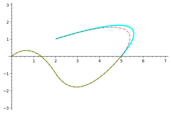
You can't concatenate Bézier paths by simply concatenating the corresponding lists. For example, let B1 and B2 be the Bézier paths generated by the lists L1=[[p1,c1,p2], [c2,p3]] and L2=[[p3,c3,p4]], and let C be the Bézier path associated to L1+L2=[[p1,c1,p2], [c2,p3], [p3,c3,p4]]. The concatenation of B1and B2 is formed by three quadratic Bézier curves. However, C is composed by two quadratic Bézier curves and a cubic one. Note that [p3,c3,p4] in L1+L2 is interpreted as a curve starting at p3 and ending at p4 which has two control points p3 and c3, so it is a cubic Bézier curve. This situation can be clearly seen in the plot generated by the following code, where B1, B2 and C are colored in green, blue and red respectively:
L1 = [[(0,0),(1,1),(2,-1)],[(3,-3),(5,0)]]
L2 = [[(5,0),(7,3),(2,1)]]
B1 = bezier_path(L1,rgbcolor="lightgreen",thickness=3)
B2 = bezier_path(L2,rgbcolor="cyan",thickness=3)
C = bezier_path(L1+L2,rgbcolor="red",linestyle="-.")
show(B1+B2+C)
In your case there is the additional problem that, due to rounding errors, both paths have different endpoints:
sage: path1[0]
Bezier path from (-1.0000000000000004, 3.3306690738754696e-16) to (1.0, -2.220446049250313e-16)
sage: path2[0]
Bezier path from (1.0000000000000002, 0.0) to (-1.0, 2.220446049250313e-16)
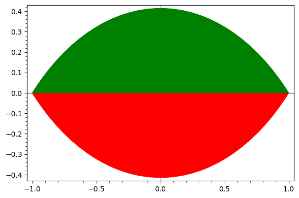
It seems that you just want to fill the region limited by both paths. You can achieve this by changing some graphic options as follows:
arc1 = arc((0,1),sqrt(2),sector=(5*pi/4,7*pi/4))
arc2 = arc((0,-1),sqrt(2),sector=(pi/4,3*pi/4))

path1 = arc1[0].bezier_path()
path2 = arc2[0].bezier_path()

opts = path1[0].options()
opts.update({"fill": True, "rgbcolor": "red"})
path1[0].set_options(opts)

opts = path2[0].options()
opts.update({"fill": True, "rgbcolor": "green"})
path2[0].set_options(opts)

show(path1 + path2, frame=True)
This is the output:
Hope this helps.
Edited (10/12/2020): An alternative route to get similar plots could be to define a function like the following one:
def circular_arc(center, radius, sector=(0,pi), segment=True,
                 plot_points=50, **kwargs):
    step = (sector[1]-sector[0])/(plot_points-1)
    pts = [(center[0]+radius*cos(t), center[1]+radius*sin(t))
           for t in [sector[0]..sector[1],step=step]]
    if(not segment): pts.append(center)
    return polygon(pts,**kwargs)
This function has a syntax similar to that of arc. It plots the circular segment determined by the arc if segment=True, or the corresponding circular sector if segment=False. With this function at hand, the following code yields almost exactly the same output as above:
arc1 = circular_arc((0,1), sqrt(2), sector=(5*pi/4,7*pi/4), color="red")
arc2 = circular_arc((0,-1), sqrt(2), sector=(pi/4,3*pi/4), color="green")
show(arc1 + arc2, frame=True, aspect_ratio=golden_ratio)
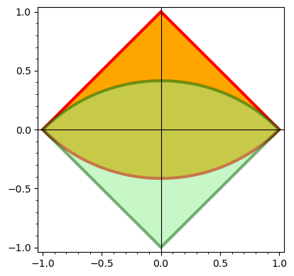
Just for the purpose of comparison, let us show what happens with segment=False:
arc1 = circular_arc((0,1), sqrt(2), sector=(5*pi/4,7*pi/4), segment=False,
                    color="orange", edgecolor="red", thickness=3)
arc2 = circular_arc((0,-1), sqrt(2), sector=(pi/4,3*pi/4), segment=False,
                    color="lightgreen", edgecolor="darkgreen",
                    thickness=3, alpha=0.5)
show(arc1 + arc2, frame=True)