Revision history [back]

I will try to answer to questions 3 and 4. I don't really know if you can directly place on the surface the level curves generated by contour_plot or put them on the $xy$ plane. It seems to me that SageMath doesn't have a command or function for doing so. In fact, the plot3d method for 2D graphics doesn't work for contour plots.

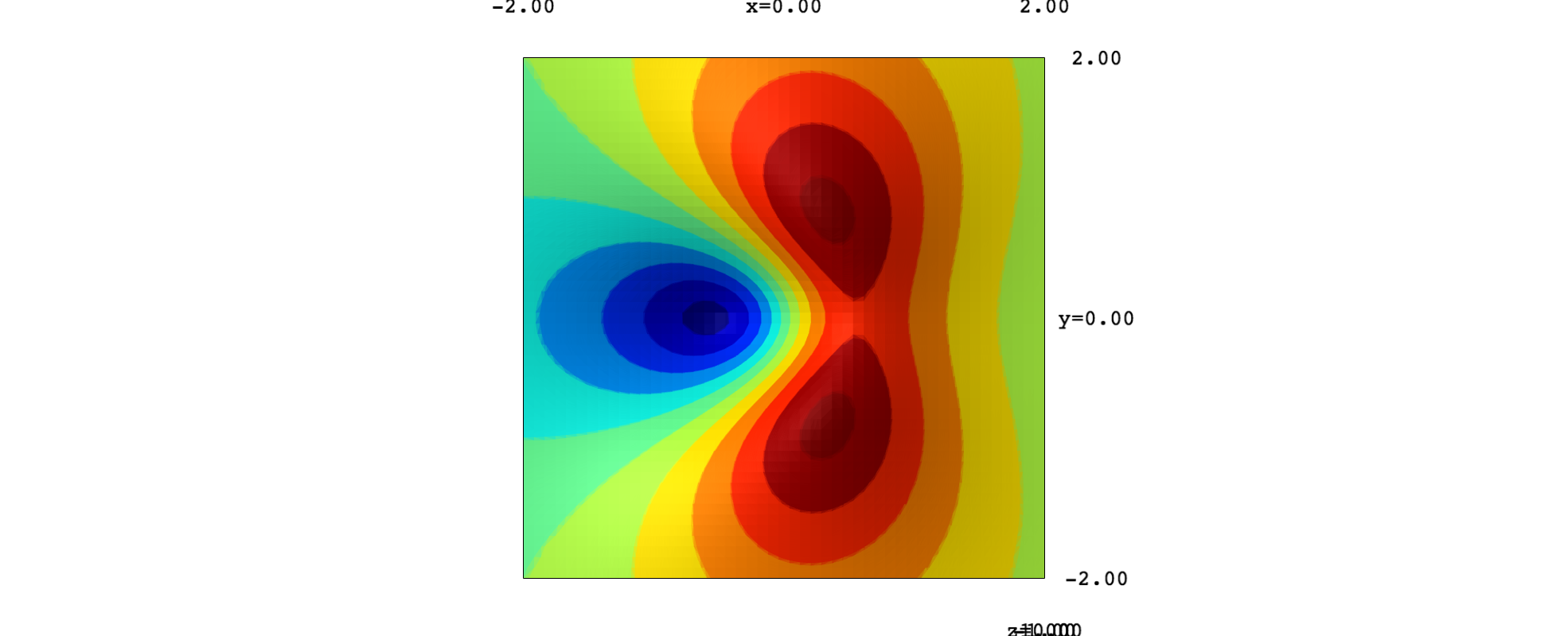
However, you can mimic the expected result by playing with colors. To exemplify the method, let us consider the function $$f(x,y) = \frac{2x+3y^2}{(x^2+y^2+1)^2}.$$ Here we have its contour plot in $[-2,2]\times[-2,2]$:

var("x,y,z")
f(x,y) = (2*x+3*y^2) / (x^2+y^2+1)^2
# Contours from z1 to z2. 
# This interval is divided into ni subintervals
z1, z2 = -0.6, 0.8
ni = 10
dz = (z2-z1)/ni
levels = [z1,z1+dz..z2]
curves = contour_plot(f(x,y), (x,-2,2), (y,-2,2), contours=levels, 
                      cmap="jet", colorbar=True)
show(curves)

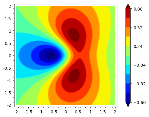
Please, note that I have explicitly provided the levels to be plotted in order to compare this figure with that of the surface.

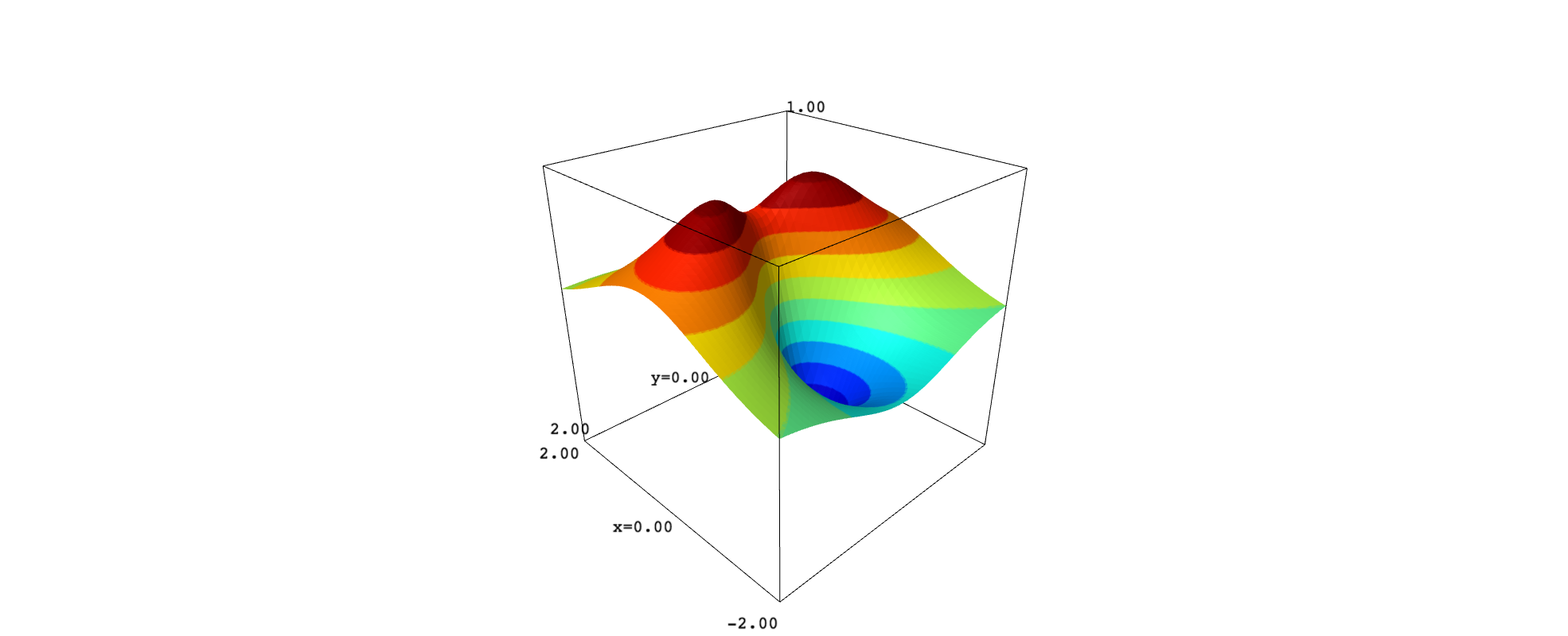
Now we plot the surface $z=f(x,y)$ using plot3d. Through a convenient definition of the color function, you can reproduce the very same contours on the surface:

# Surface plot using plot3d
def col2(x,y):
    return float(0.5*dz+floor((f(x,y)-z1)/dz)/ni)
surf = plot3d(f(x,y), (x,-2,2), (y,-2,2), color=(col2,colormaps.jet), plot_points=300)
show(surf, aspect_ratio=[1,1,2])

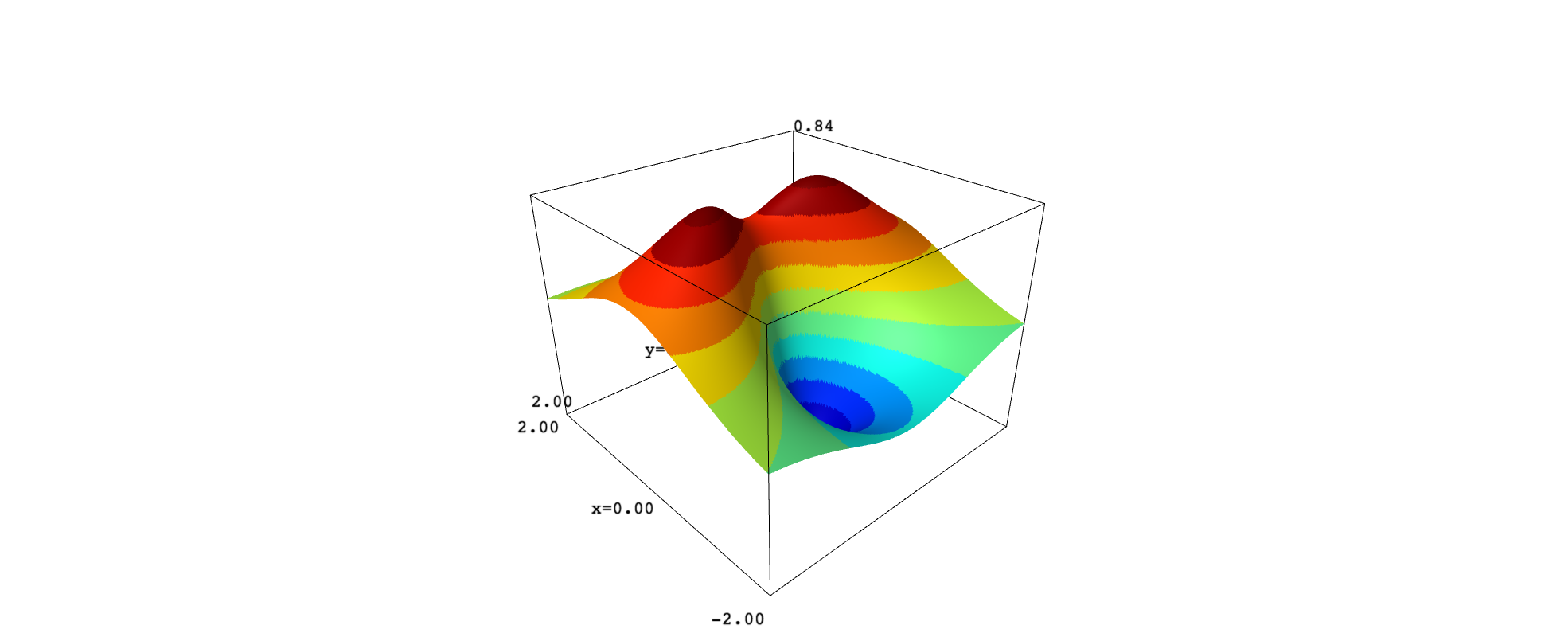
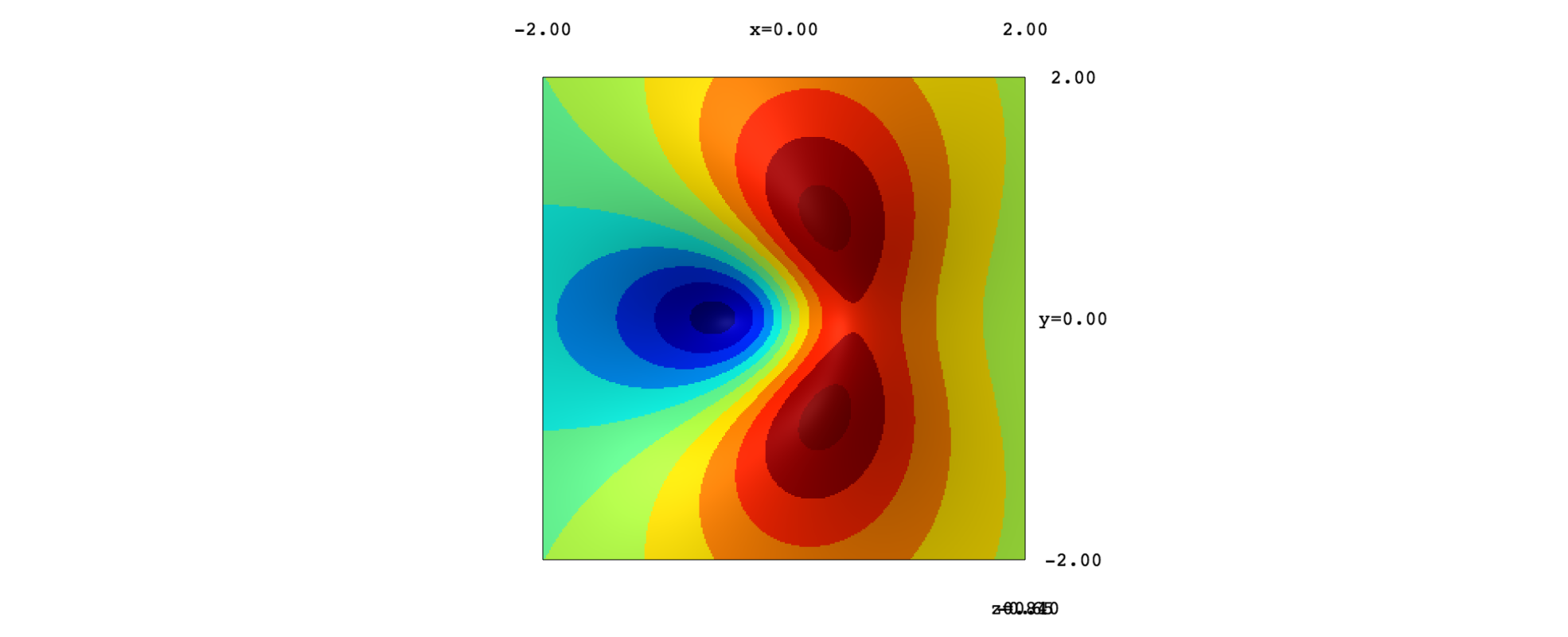
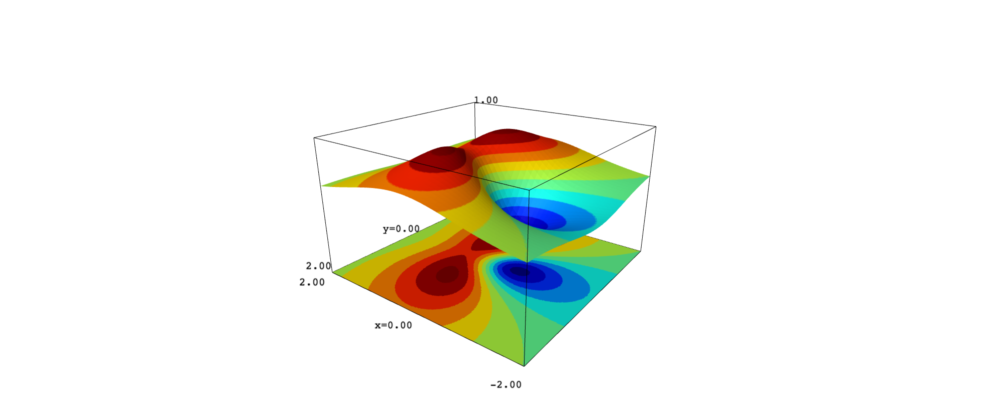
If we use an orthographic projection, we can then rotate the surface to look at it from above and compare with the contour plot:

show(surf, projection="orthographic")

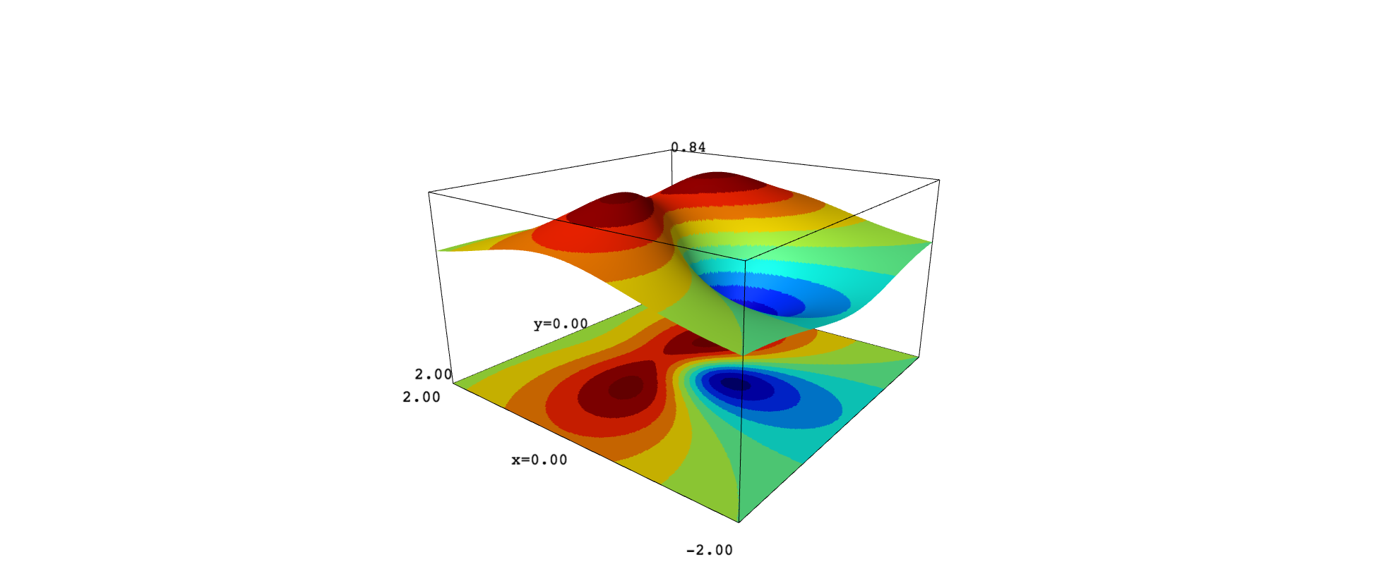
The same strategy serves to color a plane below the surface, simulating a projection of the contours on the $xy$ plane:

offset = -1.4
plane = plot3d(offset, (x,-2,2), (y,-2,2), color=(col2,colormaps.jet), plot_points=300)
show(surf+plane)

The problem with this approach is that the surface looks jagged, even using a great number of plot points. As an alternative, we can apply implicit_plot3d:

# Surface plot using implicit_plot3d
zmin, zmax = -1, 1
def col3(x,y,z):
    return float(0.5*dz+floor((z-z1)/dz)/ni)
surf_new = implicit_plot3d(z==f(x,y), (x,-2,2), (y,-2,2), (z,zmin,zmax), 
                           color=(col,colormaps.jet), plot_points=[50,50,300])
show(surf_new, aspect_ratio=[1,1,2])

Here we have again a view from above:

show(surf_new, projection="orthographic")

And the surface with the plane:

show(surf_new+plane)

It seems that implicit_plot3d provides smoother curves on the surface. To get them, it is important to use many points along the $z$-direction.