Revision history [back]

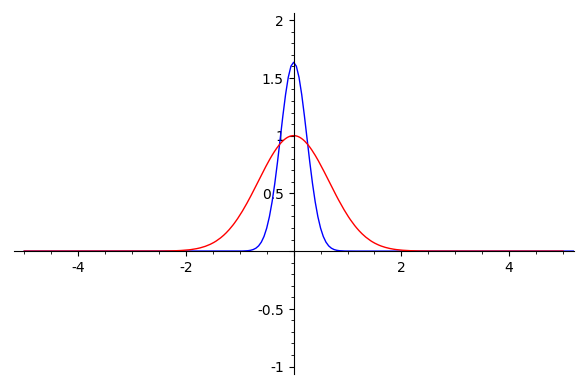
At least you can always take a naive numerical approach:

F = lambda x: exp(-x^2)*sin(x)/x
plot2 = plot(F, xmin = -5, xmax = 5, color = 'red')
### continuous Fourier transform on RR
fhat_real = lambda xi: numerical_integral(lambda x: (F(x)*exp(-2*pi*I*x*xi)).real_part(),-oo,oo, eps_abs=1e-3, eps_rel=1e-3)[0]
import numpy
plot1 = list_plot([(x,fhat_real(x)) for x in numpy.arange(-5,5, step=0.05)], plotjoined=True)
show(plot1 + plot2, xmin = -5, xmax = 5, ymin = -1, ymax = 2)

Output: