Revision history [back]
| | 1 | initial version |

I don't know how to fix that code, but as an alternative you can use desolve_system_rk4:
var('y0 y1 t')
ode_rhs = [y1, -2/t*y1 - y0^(3/2)]
points = desolve_system_rk4(ode_rhs,[y0,y1],ics=[0.1,1,0],ivar=t,end_points=10,step=0.1)
To plot y0 (i.e. $x$) against t:
ty0_points = [ [i,j] for i,j,k in points]
list_plot(ty0_points, plotjoined=True)
To plot y1 against y0 (together with the vector field):
y0y1_points = [ [j,k] for i,j,k in points]
list_plot(y0y1_points, plotjoined=True, color='red') + sum(arrow2d(p[1:], vector(p[1:]) + vector([eqn_rhs.subs({t : p[0], y0 : p[1], y1: p[2]}) for eqn_rhs in ode_rhs]).normalized()*0.03,arrowsize=1,color='blue') for p in points if p[1] >= 0)
The vector field only makes sense when y0 >= 0 (same for the ODE and its solution plotted above). I don't know what the solver does past that point; I wouldn't trust it.
| | 2 | No.2 Revision |
I don't know how to fix that code, but as an alternative you can use desolve_system_rk4:
var('y0 y1 t')
ode_rhs = [y1, -2/t*y1 - y0^(3/2)]
points = desolve_system_rk4(ode_rhs,[y0,y1],ics=[0.1,1,0],ivar=t,end_points=10,step=0.1)
To plot y0 (i.e. $x$) against t:
ty0_points = [ [i,j] for i,j,k in points]
list_plot(ty0_points, plotjoined=True)
To plot the curve in the (y0,y1 against )-plane (together with the vector field):y0
y0y1_points = [ [j,k] for i,j,k in points]
list_plot(y0y1_points, plotjoined=True, color='red') + sum(arrow2d(p[1:], vector(p[1:]) + vector([eqn_rhs.subs({t : p[0], y0 : p[1], y1: p[2]}) for eqn_rhs in ode_rhs]).normalized()*0.03,arrowsize=1,color='blue') for p in points if p[1] >= 0)
The vector field only makes sense when y0 >= 0 (same for the ODE and its solution plotted above). I don't know what the solver does past that point; I wouldn't trust it.
| | 3 | No.3 Revision |
I don't know how to fix that code, but as an alternative you can use desolve_system_rk4:
var('y0 y1 t')
ode_rhs = [y1, -2/t*y1 - y0^(3/2)]
points = desolve_system_rk4(ode_rhs,[y0,y1],ics=[0.1,1,0],ivar=t,end_points=10,step=0.1)
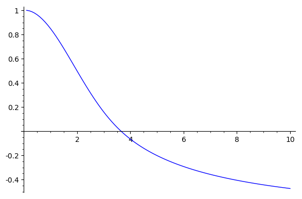
To plot y0 (i.e. $x$) against t:
ty0_points = [ [i,j] for i,j,k in points]
list_plot(ty0_points, plotjoined=True)
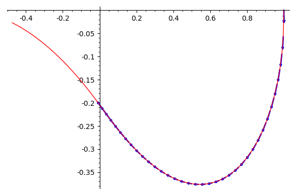
To plot the curve in the (y0,y1)-plane (together with the vector field):
y0y1_points = [ [j,k] for i,j,k in points]
list_plot(y0y1_points, plotjoined=True, color='red') + sum(arrow2d(p[1:], vector(p[1:]) + vector([eqn_rhs.subs({t : p[0], y0 : p[1], y1: p[2]}) for eqn_rhs in ode_rhs]).normalized()*0.03,arrowsize=1,color='blue') for p in points if p[1] >= 0)
The vector field only makes sense when y0 >= 0 (same for the ODE and its solution "solution" plotted above). I don't know what the solver does past that point; I wouldn't trust it.
