Revision history [back]
| | 1 | initial version |
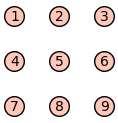
Say a graph G has nine vertices numbered 1 to 9
and we want the grid layout in the question.
One easily defines a dictionary of positions.
The set_pos method then lets us assign those
positions to the graph.
The positions can also be set when creating the
graph, using the pos=... optional argument.
For example, define the vertex set.
sage: V = [1 .. 9]
Then the position dictionary:
sage: pos = {v: (n % 3, -(n // 3)) for n, v in enumerate(V)}
Now build a graph with those vertices, no edges, and those positions:
sage: G = Graph([V, []], format='vertices_and_edges', pos=pos)
Plot it:
sage: G.plot()
If we start from an adjacency matrix, the vertices will be numbered from 0.
Start from the matrix in the question and remove one of row (chosen so the resulting matrix is symmetric):
sage: A = matrix([[1, 1, 0, 1, 0, 0, 0, 0, 0],
....:         [1, 1, 1, 0, 1, 0, 0, 0, 0],
....:         [0, 1, 1, 0, 0, 1, 0, 0, 0],
....:         [1, 0, 0, 1, 1, 0, 1, 0, 0],
....:         [1, 0, 0, 1, 1, 0, 1, 1, 0],
....:         [0, 1, 0, 1, 1, 1, 0, 1, 0],
....:         [0, 0, 1, 0, 1, 1, 0, 0, 1],
....:         [0, 0, 0, 1, 0, 0, 1, 1, 0],
....:         [0, 0, 0, 0, 1, 0, 1, 1, 1],
....:         [0, 0, 0, 0, 0, 1, 0, 1, 1]])

sage: A.nrows(), A.ncols()
(10, 9)
sage: Arows = A.rows()
sage: del Arows[4]
sage: B = matrix(Arows)
sage: B.is_symmetric()
True
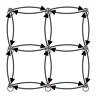
Define positions for vertices 0 to 8 and build a digraph from that matrix with those positions:
sage: pos = {n: (n % 3, -(n // 3)) for n in range(9)}
sage: D = DiGraph(B, format='adjacency_matrix', pos=pos)
sage: D.plot()
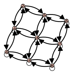
Note that without setting the positions ourselves, the default "spring" layout algorithm would already do a very good job on the grid graph, starting from the corrected matrix.
sage: D = DiGraph(B, format='adjacency_matrix)  # don't set pos
sage: D.plot()
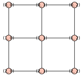
Note that Sage also offers a GridGraph constructor
which labels the vertices with their coordinates
and positions them in a grid by itself.
sage: G = graphs.GridGraph((3, 3))
sage: G.plot()
Regarding colouring options, the documentations has plenty of examples, and there have also been many questions and answers on Ask Sage which provide nice examples.
| | 2 | No.2 Revision |
Say a graph G has nine vertices numbered 1 to 9
and we want the grid layout in the question.
One easily defines a dictionary of positions.
The set_pos method then lets us assign those
positions to the graph.
The positions can also be set when creating the
graph, using the pos=... optional argument.
For example, define the vertex set.
sage: V = [1 .. 9]
Then the position dictionary:
sage: pos = {v: (n % 3, -(n // 3)) for n, v in enumerate(V)}
Now build a graph with those vertices, no edges, and those positions:
sage: G = Graph([V, []], format='vertices_and_edges', pos=pos)
Plot it:
sage: G.plot()
If we start from an adjacency matrix, the vertices will be numbered from 0.
Start from the matrix in the question and remove one of row (chosen so the resulting matrix is symmetric):
sage: A = matrix([[1, 1, 0, 1, 0, 0, 0, 0, 0],
....:         [1, 1, 1, 0, 1, 0, 0, 0, 0],
....:         [0, 1, 1, 0, 0, 1, 0, 0, 0],
....:         [1, 0, 0, 1, 1, 0, 1, 0, 0],
....:         [1, 0, 0, 1, 1, 0, 1, 1, 0],
....:         [0, 1, 0, 1, 1, 1, 0, 1, 0],
....:         [0, 0, 1, 0, 1, 1, 0, 0, 1],
....:         [0, 0, 0, 1, 0, 0, 1, 1, 0],
....:         [0, 0, 0, 0, 1, 0, 1, 1, 1],
....:         [0, 0, 0, 0, 0, 1, 0, 1, 1]])

sage: A.nrows(), A.ncols()
(10, 9)
sage: Arows = A.rows()
sage: del Arows[4]
sage: B = matrix(Arows)
sage: B.is_symmetric()
True
Define positions for vertices 0 to 8 and build a digraph from that matrix with those positions:
sage: pos = {n: (n % 3, -(n // 3)) for n in range(9)}
sage: D = DiGraph(B, format='adjacency_matrix', pos=pos)
sage: D.plot()
Note that without setting the positions ourselves, the default "spring" layout algorithm would already do a very good job on the grid graph, starting from the corrected matrix.
sage: D = DiGraph(B, format='adjacency_matrix)  # don't set pos
sage: D.plot()
Note that The positions have not been set at the time of creating this graph.
Defines pos as above, and running
sage: D.set_pos(pos)
sage: D.plot()
gives the same output as when we defined D = DiGraph(..., pos=pos) above.
Sage also offers has a built-in GridGraph constructor
constructor which labels the vertices with vertices
by their coordinates
coordinates and positions them in a grid all by itself.
sage: G = graphs.GridGraph((3, 3))
sage: G.plot()
Regarding colouring options, the documentations has plenty of examples, and there have also been many questions and answers on Ask Sage which provide nice examples.
| | 3 | No.3 Revision |
Say a graph G has nine vertices numbered 1 to 9
and we want the grid layout in the question.
One easily defines a dictionary of positions.
The set_pos method then lets us assign those
positions to the graph.
The positions can also be set when creating the
graph, using the pos=... optional argument.
For example, define the vertex set.
sage: V = [1 .. 9]
Then the position dictionary:
sage: pos = {v: (n % 3, -(n // 3)) for n, v in enumerate(V)}
Now build a graph with those vertices, no edges, and those positions:
sage: G = Graph([V, []], format='vertices_and_edges', pos=pos)
Plot it:
sage: G.plot()
If we start from an adjacency matrix, the vertices will be numbered from 0.
Start from the matrix in the question and remove one of row (chosen so the resulting matrix is symmetric):
sage: A = matrix([[1, 1, 0, 1, 0, 0, 0, 0, 0],
....:         [1, 1, 1, 0, 1, 0, 0, 0, 0],
....:         [0, 1, 1, 0, 0, 1, 0, 0, 0],
....:         [1, 0, 0, 1, 1, 0, 1, 0, 0],
....:         [1, 0, 0, 1, 1, 0, 1, 1, 0],
....:         [0, 1, 0, 1, 1, 1, 0, 1, 0],
....:         [0, 0, 1, 0, 1, 1, 0, 0, 1],
....:         [0, 0, 0, 1, 0, 0, 1, 1, 0],
....:         [0, 0, 0, 0, 1, 0, 1, 1, 1],
....:         [0, 0, 0, 0, 0, 1, 0, 1, 1]])

sage: A.nrows(), A.ncols()
(10, 9)
sage: Arows = A.rows()
sage: del Arows[4]
sage: B = matrix(Arows)
sage: B.is_symmetric()
True
Define positions for vertices 0 to 8 and build a digraph from that matrix with those positions:
sage: pos = {n: (n % 3, -(n // 3)) for n in range(9)}
sage: D = DiGraph(B, format='adjacency_matrix', pos=pos)
sage: D.plot()
Note that without setting the positions ourselves, the default "spring" layout algorithm would already do a very good job on the grid graph, starting from the corrected matrix.
sage: D = DiGraph(B, format='adjacency_matrix)  # don't set pos
sage: D.plot()
The positions have not been set at the time of creating this graph.
Defines pos as above, and running
sage: D.set_pos(pos)
sage: D.plot()
gives the same output as when we defined D = DiGraph(..., pos=pos) above.
Sage has a built-in GridGraph constructor which labels the vertices
by their coordinates and positions them in a grid all by itself.
sage: G = graphs.GridGraph((3, 3))
sage: G.plot()
This gives an undirected graph.
Turning it into a directed graph is easy:
sage: D = DiGraph(G)
This preserves the positions!
One can also relabel the vertices:
sage: D.relabel([1 .. 9])
This also preserves the positions!
To sum up, the easiest way to achieve the graph in the question might be:
sage: D = DiGraph(graphs.GridGraph((3, 3)), loops=True)
sage: D.relabel([1 .. 9])
sage: D.add_edges((i, i) for i in D.vertices())
sage: D
Regarding colouring options, the documentations has plenty the customisation of examples,
vertex and there have also been edges labels,
start by checking the documentation and/or the many questions questions
and answers on Ask Sage which
which provide nice instructive examples.
