Revision history [back]
| | 1 | initial version | |

Motivated by @slelievre's answer, I'm going to provide an alternative solution based on Bézier patches, which also answers this related question: Concatenate Bézier paths?
Bézier paths
Let us start by considering some facts about Bézier paths. They result from the concatenation of several linear, quadratic or cubic Bézier curves. In SageMath, Bézier paths can be obtained with the bezier_path function, as shown here:
bpath = [[(2,1),(1,0),(0,1),(1,3)], [(2,5)], [(4,9),(4,2)]]
foo = bezier_path(bpath)
show(foo, frame=True, axes=False)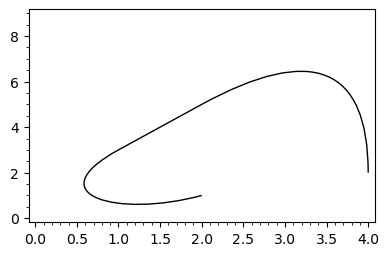
The argument of bezier_path is a list of lists; except the first one, each list contains the control points and the end point of the corresponding Bézier curve, the start point being the end point of the preceding curve. This function returns a Graphics object, which wraps a BezierPath object:
sage: type(foo)
<class 'sage.plot.graphics.Graphics'>
sage: type(foo[0])
<class 'sage.plot.bezier_path.BezierPath'>
Once obtained a Bézier path, suppose that we delete the list that generated it. Can we recover such a list if we need it again? Yes, we can do it by using the vertices and codes methods defined by the BezierPath class:
sage: foo[0].vertices
array([[2., 1.],
       [1., 0.],
       [0., 1.],
       [1., 3.],
       [2., 5.],
       [4., 9.],
       [4., 2.]])
sage: foo[0].codes
[1, 4, 4, 4, 2, 3, 3]
As we can see, vertices yields a Numpy array which contains all the points involved in the generation of the Bézier path, whereas codes provides a list whose first element is always 1; the remaining elements say the order of the Bézier curve to which its associated point belongs. Please note that the first point in each curve (except the first one) is omitted. The following code allows to recover the argument of bezier_path from vertices and codes:
def recover_bpath(ver, cod):
    ii = len(cod)-1
    bpath = []
    while ii > 0:
        cc = cod[ii]
        bpath = [ ver[ii-cc+2:ii+1] ] + bpath
        ii -= cc-1
    bpath[0] = [ver[0]] + bpath[0]
    return bpath
To test this function, let us construct the list that generated foo:
sage: ver, cod = foo[0].vertices.tolist(), foo[0].codes
sage: recover_bpath(ver,cod)
[[[2.0, 1.0], [1.0, 0.0], [0.0, 1.0], [1.0, 3.0]],
 [[2.0, 5.0]],
 [[4.0, 9.0], [4.0, 2.0]]]
Here tolist serves to convert the Numpy array into a list.
It is now easy to concatenate Bézier paths, since it suffices to suitably merge their corresponding vertices and codes. We have to consider two cases, depending on whether the end point of the first path is the start point of the second path or not. This is done by the following function, whose two arguments are lists of the form [vertices, codes]:
def concatenate_bpaths(bp1, bp2, tolerance=1e-10):
    if bp1==[]: return bp2
    v1, c1 = bp1
    v2, c2 = bp2
    if norm(vector(v1[-1])-vector(v2[0]))<tolerance:
        # end point first path = start point second path
        c = c1 + c2[1:]
        v = v1 + v2[1:]
    else:
        # end point first path != start point second path
        c = c1 + [2] + c2[1:]
        v = v1 + v2
    return v, c
Note that, due to rounding errors, two points are considered equal if their distance is small enough. Let us now use these functions to graphically concatenate Bézier paths:
# Bézier paths used in this example
bp1 = [[(3,1),(1,1),(1,3),(2,4)], [(4,6)], [(5,7),(7,5)]]
bp2 = [[(7,5),(9,3),(7,2)],[(3,0),(6,-1)]]
bp3 = [[(3,0),(6,-2),(7,-1)],[(9,1),(6,1)]]
BP1 = bezier_path(bp1, color="red")
BP2 = bezier_path(bp2, color="green")
BP3 = bezier_path(bp3, color="blue")
# Vertices and codes of each Bezier path
v1, c1 = BP1[0].vertices.tolist(), BP1[0].codes
v2, c2 = BP2[0].vertices.tolist(), BP2[0].codes
v3, c3 = BP3[0].vertices.tolist(), BP3[0].codes
# Concatenate BP1 and BP2
v12, c12 = concatenate_bpaths([v1,c1], [v2,c2])
bp12 = recover_bpath(v12,c12)
BP12 = bezier_path(bp12, color="gray")
# Concatenate BP3 and BP1
v31, c31 = concatenate_bpaths([v3,c3], [v1,c1])
bp31 = recover_bpath(v31,c31)
BP31 = bezier_path(bp31, color="gray")
# Show all the paths
graphics_array([[BP1+BP2,BP12],[BP3+BP1,BP31]]).show(frame=True, axes=False)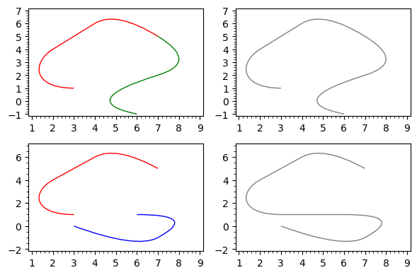
Likewise, given the vertices and codes of a Bézier path, we can easily get the vertices and codes of the same path but travelled in the opposite direction, allowing to reverse the start and end points of the path:
def reverse_bpath(ver,cod):
    return ver[::-1], [1] + cod[:0:-1]
Bézier paths for arcs and lines. Hyperbolic polygons
The line graphics primitive yields (poly)lines, which can be considered particular cases of Bézier paths, since a segment is a linear Bézier curve. Likewise, the arc primitive provides circular arcs, which can be approximated with a Bézier path. In fact, such a path is provided by the bezier_path method of the Arc class. The advantage of using Bézier paths instead of the original graphics primitives is that Bézier paths can be concatenated. A closed Bézier path can also be filled. So, given a Line or Arc object, let us see how we can get the vertices and codes of the associated Bézier path:
def get_bpath(object):
    if isinstance(object,sage.plot.line.Line):
        ver = [(x,y) for x,y in zip(object.xdata,object.ydata)]
        cod = [1] + (len(object.xdata)-1)*[2]
    elif isinstance(object,sage.plot.arc.Arc):
        b = object.bezier_path()[0]
        ver, cod = reverse_bpath(b.vertices.tolist(), b.codes)
    else:
        raise TypeError("The argument is not a Line nor an Arc instance")
    return ver, cod
By default, the Bézier path for an Arc object is travelled counterclockwise. But we need the opposite orientation in order to construct hyperbolic polygons. This is why such a path has been reversed in the preceding function definition.
As shown by @slelievre in his answer, when using the Poincaré disk model, geodesics in the hyperbolic plane are arcs or lines. Hence, to concatenate geodesics and form hyperbolic polygons, we can manipulate their equivalent Bézier paths. This leads to the following function, called disk_ngon, which borrows inspiration, code and (almost) the name from the disc_ngon function defined by @slelievre:
def disk_ngon(points, alpha=1, color='darkgreen', fill_color='lightgreen', linestyle='solid',
              thickness=1.5, zorder=2, tolerance=1e-10, **opt):
    line_opt = {'alpha': alpha, 'fill': False, 'color': color,
                'thickness': thickness, 'zorder': zorder, 'linestyle': linestyle}
    fill_opt = {'alpha': alpha, 'fill': True, 'color': fill_color,
                'thickness': 0, 'zorder': zorder}
    n = len(points)
    if n < 3:
        raise ValueError(f"Need >= 3 points for polygon, got {n}")
    DD = HyperbolicPlane().PD()

    bp_all = []
    for k, q in enumerate(points, start=-1):
        p = points[k]
        pq = DD.get_geodesic(p, q).plot()
        bp_pq = get_bpath(pq[0])
        bp_all = concatenate_bpaths(bp_all, bp_pq, tolerance=tolerance)

    bpath = recover_bpath(*bp_all)
    contour = bezier_path(bpath, **line_opt)
    inside = bezier_path(bpath, **fill_opt)
    return inside + DD.get_background_graphic(**opt) + contour
For the sake of brevity, I have omitted the docstring, which should be almost identical to that of disc_ngon. Here we have the same examples provided by @slelievre, with small graphic variants:
a = [1, I, -1]
b = [0, 1/2, 1/2 + 1/2*I, 1/2*I]
c = [0, 1/2, 1/2 + 1/2*I, I, -1/2 + 1/2*I]
d = [(3/4 if k % 2 else 1)*E(8)^k for k in range(8)]
abcd = [disk_ngon(p) for p in [a, b, c, d]]
graphics_array([abcd[:2],abcd[2:]]).show(figsize=6)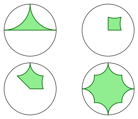
fives = [[r/4*E(5)^k for k in range(5)] for r in range(1, 5)]
fivegons = [disk_ngon(f) for f in fives]
graphics_array([fivegons[:2],fivegons[2:]]).show(figsize=6)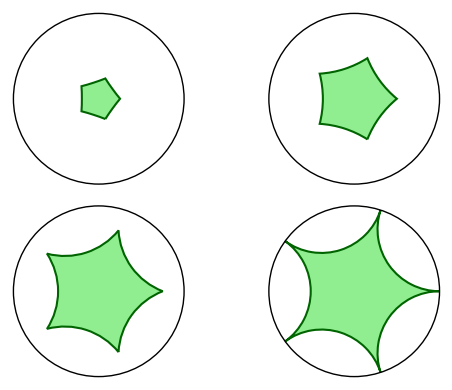
| | 2 | No.2 Revision |
Motivated by @slelievre's answer, I'm going to provide an alternative solution based on Bézier patches, paths, which also answers this related question: Concatenate Bézier paths?
Bézier paths
Let us start by considering some facts about Bézier paths. They result from the concatenation of several linear, quadratic or cubic Bézier curves. In SageMath, Bézier paths can be obtained with the bezier_path function, as shown here:
bpath = [[(2,1),(1,0),(0,1),(1,3)], [(2,5)], [(4,9),(4,2)]]
foo = bezier_path(bpath)
show(foo, frame=True, axes=False)
The argument of bezier_path is a list of lists; except the first one, each list contains the control points and the end point of the corresponding Bézier curve, the start point being the end point of the preceding curve. This function returns a Graphics object, which wraps a BezierPath object:
sage: type(foo)
<class 'sage.plot.graphics.Graphics'>
sage: type(foo[0])
<class 'sage.plot.bezier_path.BezierPath'>
Once obtained a Bézier path, suppose that we delete the list that generated it. Can we recover such a list if we need it again? Yes, we can do it by using the vertices and codes methods defined by the BezierPath class:
sage: foo[0].vertices
array([[2., 1.],
       [1., 0.],
       [0., 1.],
       [1., 3.],
       [2., 5.],
       [4., 9.],
       [4., 2.]])
sage: foo[0].codes
[1, 4, 4, 4, 2, 3, 3]
As we can see, vertices yields a Numpy array which contains all the points involved in the generation of the Bézier path, whereas codes provides a list whose first element is always 1; the remaining elements say the order of the Bézier curve to which its associated point belongs. Please note that the first point in each curve (except the first one) is omitted. The following code allows to recover the argument of bezier_path from vertices and codes:
def recover_bpath(ver, cod):
    ii = len(cod)-1
    bpath = []
    while ii > 0:
        cc = cod[ii]
        bpath = [ ver[ii-cc+2:ii+1] ] + bpath
        ii -= cc-1
    bpath[0] = [ver[0]] + bpath[0]
    return bpath
To test this function, let us construct the list that generated foo:
sage: ver, cod = foo[0].vertices.tolist(), foo[0].codes
sage: recover_bpath(ver,cod)
[[[2.0, 1.0], [1.0, 0.0], [0.0, 1.0], [1.0, 3.0]],
 [[2.0, 5.0]],
 [[4.0, 9.0], [4.0, 2.0]]]
Here tolist serves to convert the Numpy array into a list.
It is now easy to concatenate Bézier paths, since it suffices to suitably merge their corresponding vertices and codes. We have to consider two cases, depending on whether the end point of the first path is the start point of the second path or not. This is done by the following function, whose two arguments are lists of the form [vertices, codes]:
def concatenate_bpaths(bp1, bp2, tolerance=1e-10):
    if bp1==[]: return bp2
    v1, c1 = bp1
    v2, c2 = bp2
    if norm(vector(v1[-1])-vector(v2[0]))<tolerance:
        # end point first path = start point second path
        c = c1 + c2[1:]
        v = v1 + v2[1:]
    else:
        # end point first path != start point second path
        c = c1 + [2] + c2[1:]
        v = v1 + v2
    return v, c
Note that, due to rounding errors, two points are considered equal if their distance is small enough. Let us now use these functions to graphically concatenate Bézier paths:
# Bézier paths used in this example
bp1 = [[(3,1),(1,1),(1,3),(2,4)], [(4,6)], [(5,7),(7,5)]]
bp2 = [[(7,5),(9,3),(7,2)],[(3,0),(6,-1)]]
bp3 = [[(3,0),(6,-2),(7,-1)],[(9,1),(6,1)]]
BP1 = bezier_path(bp1, color="red")
BP2 = bezier_path(bp2, color="green")
BP3 = bezier_path(bp3, color="blue")
# Vertices and codes of each Bezier path
v1, c1 = BP1[0].vertices.tolist(), BP1[0].codes
v2, c2 = BP2[0].vertices.tolist(), BP2[0].codes
v3, c3 = BP3[0].vertices.tolist(), BP3[0].codes
# Concatenate BP1 and BP2
v12, c12 = concatenate_bpaths([v1,c1], [v2,c2])
bp12 = recover_bpath(v12,c12)
BP12 = bezier_path(bp12, color="gray")
# Concatenate BP3 and BP1
v31, c31 = concatenate_bpaths([v3,c3], [v1,c1])
bp31 = recover_bpath(v31,c31)
BP31 = bezier_path(bp31, color="gray")
# Show all the paths
graphics_array([[BP1+BP2,BP12],[BP3+BP1,BP31]]).show(frame=True, axes=False)
Likewise, given the vertices and codes of a Bézier path, we can easily get the vertices and codes of the same path but travelled in the opposite direction, allowing to reverse the start and end points of the path:
def reverse_bpath(ver,cod):
    return ver[::-1], [1] + cod[:0:-1]
Bézier paths for arcs and lines. Hyperbolic polygons
The line graphics primitive yields (poly)lines, which can be considered particular cases of Bézier paths, since a segment is a linear Bézier curve. Likewise, the arc primitive provides circular arcs, which can be approximated with a Bézier path. In fact, such a path is provided by the bezier_path method of the Arc class. The advantage of using Bézier paths instead of the original graphics primitives is that Bézier paths can be concatenated. A closed Bézier path can also be filled. So, given a Line or Arc object, let us see how we can get the vertices and codes of the associated Bézier path:
def get_bpath(object):
    if isinstance(object,sage.plot.line.Line):
        ver = [(x,y) for x,y in zip(object.xdata,object.ydata)]
        cod = [1] + (len(object.xdata)-1)*[2]
    elif isinstance(object,sage.plot.arc.Arc):
        b = object.bezier_path()[0]
        ver, cod = reverse_bpath(b.vertices.tolist(), b.codes)
    else:
        raise TypeError("The argument is not a Line nor an Arc instance")
    return ver, cod
By default, the Bézier path for an Arc object is travelled counterclockwise. But we need the opposite orientation in order to construct hyperbolic polygons. This is why such a path has been reversed in the preceding function definition.
As shown by @slelievre in his answer, when using the Poincaré disk model, geodesics in the hyperbolic plane are arcs or lines. Hence, to concatenate geodesics and form hyperbolic polygons, we can manipulate their equivalent Bézier paths. This leads to the following function, called disk_ngon, which borrows inspiration, code and (almost) the name from the disc_ngon function defined by @slelievre:
def disk_ngon(points, alpha=1, color='darkgreen', fill_color='lightgreen', linestyle='solid',
              thickness=1.5, zorder=2, tolerance=1e-10, **opt):
    line_opt = {'alpha': alpha, 'fill': False, 'color': color,
                'thickness': thickness, 'zorder': zorder, 'linestyle': linestyle}
    fill_opt = {'alpha': alpha, 'fill': True, 'color': fill_color,
                'thickness': 0, 'zorder': zorder}
    n = len(points)
    if n < 3:
        raise ValueError(f"Need >= 3 points for polygon, got {n}")
    DD = HyperbolicPlane().PD()

    bp_all = []
    for k, q in enumerate(points, start=-1):
        p = points[k]
        pq = DD.get_geodesic(p, q).plot()
        bp_pq = get_bpath(pq[0])
        bp_all = concatenate_bpaths(bp_all, bp_pq, tolerance=tolerance)

    bpath = recover_bpath(*bp_all)
    contour = bezier_path(bpath, **line_opt)
    inside = bezier_path(bpath, **fill_opt)
    return inside + DD.get_background_graphic(**opt) + contour
For the sake of brevity, I have omitted the docstring, which should be almost identical to that of disc_ngon. Here we have the same examples provided by @slelievre, with small graphic variants:
a = [1, I, -1]
b = [0, 1/2, 1/2 + 1/2*I, 1/2*I]
c = [0, 1/2, 1/2 + 1/2*I, I, -1/2 + 1/2*I]
d = [(3/4 if k % 2 else 1)*E(8)^k for k in range(8)]
abcd = [disk_ngon(p) for p in [a, b, c, d]]
graphics_array([abcd[:2],abcd[2:]]).show(figsize=6)
fives = [[r/4*E(5)^k for k in range(5)] for r in range(1, 5)]
fivegons = [disk_ngon(f) for f in fives]
graphics_array([fivegons[:2],fivegons[2:]]).show(figsize=6)
