Revision history [back]
| | 1 | initial version |
Plot several functions together
Answer to question 1, following @FrédéricC's suggestion.
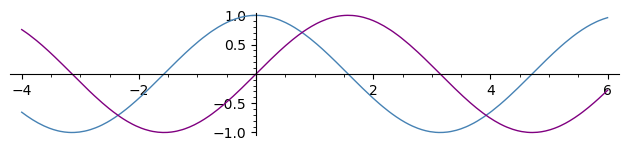
Summing individual plots:
sage: pcos = plot(cos, (-4, 6), color='steelblue')
sage: psin = plot(sin, (-4, 6), color='purple')
sage: pcos + psin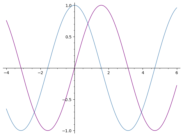
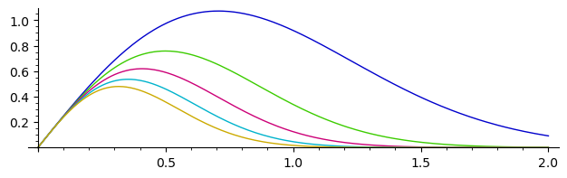
Plotting several functions together (see SageMath documentation on 2D plotting):
sage: plot([x*exp(-n*x^2)/.4 for n in [1 .. 5]], (0, 2), aspect_ratio=.8)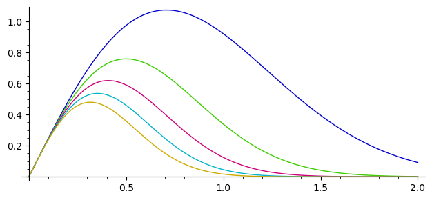
Work around tick label rendering bug
Answer to question 2.
Until the bug is fixed, a workaround is to plot with a frame, which will indicate the scaling.
Compare:
sage: p = plot(lambda x: 8e6*x); p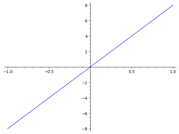
sage: q = plot(lambda x: 8e6*x, frame=True); q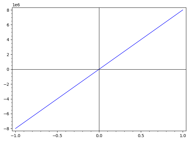
Or you could use the get_minmax_data method to get the
xmin, xmax, ymin, ymax, and somehow add them to the picture as text.
sage: d = p.get_minmax_data()
sage: xa, xb, ya, yb = d['xmin'], d['xmax'], d['ymin'], d['ymax']
sage: xc, yc = mean([xa, xa, xb]), mean([ya, ya, yb])
sage: txa = text(f"xmin:\n{xa}", (xa, yc), horizontal_alignment='left')
sage: txb = text(f"xmax:\n{xb}", (xb, yc), horizontal_alignment='right')
sage: tya = text(f"ymin:\n{ya}", (xc, ya), vertical_alignment='bottom')
sage: tyb = text(f"ymax:\n{yb}", (xc, yb), vertical_alignment='top')
sage: pt = p + sum([txa, txb, tya, tyb])
sage: pt
Launched png viewer for Graphics object consisting of 5 graphics primitives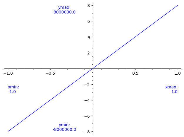
Rounding errors in floating-point calculations
Answer to question 3.
General suggestion: use Arb for arbitrary precision calculations.
In Sage, Arb can be used via RealBallField and ComplexBallField.
Search the Sage documentation or Ask Sage for examples.
| | 2 | No.2 Revision |
Plot several functions together
Answer to
This answers question 1, following @FrédéricC's suggestion.suggestions.
Summing individual plots:
sage: pcos = plot(cos, (-4, 6), color='steelblue')
sage: psin = plot(sin, (-4, 6), color='purple')
sage: pcos + psin
(pcos + psin).show(aspect_ratio=1)
Plotting several functions together (see SageMath documentation on 2D plotting):
sage: plot([x*exp(-n*x^2)/.4 for n in [1 .. 5]], (0, 2), aspect_ratio=.8)
Work around aspect_ratio=.5)
Tick label rendering bug
This answers question 2.
This bug was also reported as
Solving that problem is now tracked at
Answer to question 2.
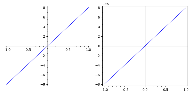
Until the bug is fixed, a workaround is to plot with a frame, which will indicate the scaling.
Compare:
sage: p = plot(lambda x: 8e6*x); p
sage: q = plot(lambda x: 8e6*x, frame=True); qsage: graphics_array([p, q]).show(figsize=(8, 4))
Or you could use the get_minmax_data method to get the
xmin, xmax, ymin, ymax, and somehow add them to the picture as text.
sage: d = p.get_minmax_data()
sage: xa, xb, ya, yb = d['xmin'], d['xmax'], d['ymin'], d['ymax']
sage: xc, yc = mean([xa, xa, xb]), mean([ya, ya, yb])
sage: txa = text(f"xmin:\n{xa}", (xa, yc), horizontal_alignment='left')
sage: txb = text(f"xmax:\n{xb}", (xb, yc), horizontal_alignment='right')
sage: tya = text(f"ymin:\n{ya}", (xc, ya), vertical_alignment='bottom')
sage: tyb = text(f"ymax:\n{yb}", (xc, yb), vertical_alignment='top')
sage: pt = p + sum([txa, txb, tya, tyb])
sage: pt
Launched png viewer for Graphics object consisting of 5 graphics primitives
Rounding errors in floating-point calculations
Answer to
This answers question 3.
General suggestion:
Problematic plot
The exponential function on [0, 1], rescaled to [-1, 1].
sage: h(x) = exp(x/2 + 1/2)Its Chebyshev approximation of order 11:
sage: f(x) = 1.648721270700127734695199 + 0.8243606353500639704213267*x + 0.2060901588375456897278408*x^2 + 0.03434835980625555348009372*x^3 + 0.004293544975435477755738488*x^4 + 0.0004293544975550920330337524*x^5 + 3.577954294118110098524956e-05*x^6 + 2.555681612268918733452545e-06*x^7 + 1.597272498430465439987321e-07*x^8 + 8.873762489265668731711247e-09*x^9 + 4.462222789173961848447732e-10*x^10 + 2.027323563290198480646098e-11*x^11The quality-of-approximation function: their difference:
sage: g(x) = f(x) - h(x)The problematic plot:
sage: pg = plot(g, color='steelblue')
sage: pg.show(frame=True, figsize=(7, 2))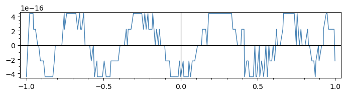
Plotting uses floating-point computations!
The plot in the question seems to be taking only 7 y-values.
This plot's goal is to visualise a quality of approximation
by plotting the difference f(x) - h(x) of two almost-equal
functions (f is an approximation of h of high quality).
Of course, this means the function g = f - h takes extremely
small values. The way they are computed becomes important!
Knowing how the plot command works helps understand
what is going on: it samples 200 floating-point values in the
plotting interval and computes the value of the function at
these points. These are floating-point computations, with
53 bits of precision, which is roughly 15 or 16 decimal digits.
Here, both f and h have values that are roughly on the
order of one, and their difference is on the order of 1e-16.
(Furthermore f itself is a polynomial, so each f(x) is
a linear combination of twelve powers of x.)
In the end each g(x) is the sum of terms of various sizes,
summed in a certain order, resulting in a value very close
to the precision of some of the numbers being summed.
It becomes hard to put much trust our output.
Arb to the rescue
A general suggestion for dealing with precision issues is to use Arb for arbitrary precision calculations.
In Sage, Arb can be used via RealBallField and ComplexBallField.
Search the The Sage documentation or and Ask Sage have a few examples.
For the purpose of this question, we can use evaluation of polynomials with integer or rational coefficients on real or complex balls. This is a recent feature of Arb, even more recently available in Sage (thanks to the work at Sage Trac ticket 30652) In fact it is only part of Sage since version 9.3.beta0.
Here is one way to use that.
Define the coefficients of the Chebyshev polynomial approximation.
sage: cc = (1.648721270700127734695199,
....:       0.8243606353500639704213267,
....:       0.2060901588375456897278408,
....:       0.03434835980625555348009372,
....:       0.004293544975435477755738488,
....:       0.0004293544975550920330337524,
....:       3.577954294118110098524956e-05,
....:       2.555681612268918733452545e-06,
....:       1.597272498430465439987321e-07,
....:       8.873762489265668731711247e-09,
....:       4.462222789173961848447732e-10,
....:       2.027323563290198480646098e-11)
Turn them into rationals:
sage: ccc = [QQ(c.as_integer_ratio()) for examples. c in cc]Define the polynomial ring over QQ with variable x:
sage: P = QQ['x']Define the quality-of-approximation function:
sage: def gg(x):
....:     return ff(x) - exp(x/2 + 1/2)
Define a real ball field with sufficient precision (here we take 1000 bits).
sage: R = RealBallField(1000)Define an alternative version of the quality-of-approximation function using real balls:
sage: def ggg(x):
....:     return gg(R(x))
Plot:
sage: pggg = plot(ggg, color='purple)
sage: pggg.show(frame=True, figsize=(7, 2))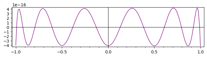
Compare to the original plot:
sage: p = plot(f(x) - exp(x/2 + 1/2), x, frame=True, figsize=(7, 2))
sage: q = plot(gg, color='steelblue', frame=True, figsize=(7, 2))
sage: (p + q).show(figsize=(7, 2))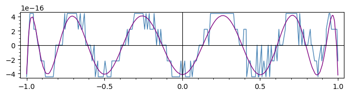
This comparison shows that despite its jaggedness, the low-resolution plot was still giving an indication of the variations of the difference between the approximating and the approximated functions.
| | 3 | No.3 Revision |
Plot several functions together
This answers question 1, following @FrédéricC's suggestions.
Summing individual plots:
sage: pcos = plot(cos, (-4, 6), color='steelblue')
sage: psin = plot(sin, (-4, 6), color='purple')
sage: (pcos + psin).show(aspect_ratio=1)
Plotting several functions together (see SageMath documentation on 2D plotting):
sage: plot([x*exp(-n*x^2)/.4 for n in [1 .. 5]], (0, 2), aspect_ratio=.5)
Tick label rendering bug
This answers question 2.
This bug was also reported as
Solving that problem is now tracked at
Until the bug is fixed, a workaround is to plot with a frame, which will indicate the scaling.
Compare:
sage: p = plot(lambda x: 8e6*x); p
sage: q = plot(lambda x: 8e6*x, frame=True); q
sage: graphics_array([p, q]).show(figsize=(8, 4))
Or you could use the get_minmax_data method to get the
xmin, xmax, ymin, ymax, and somehow add them to the picture as text.
sage: d = p.get_minmax_data()
sage: xa, xb, ya, yb = d['xmin'], d['xmax'], d['ymin'], d['ymax']
sage: xc, yc = mean([xa, xa, xb]), mean([ya, ya, yb])
sage: txa = text(f"xmin:\n{xa}", (xa, yc), horizontal_alignment='left')
sage: txb = text(f"xmax:\n{xb}", (xb, yc), horizontal_alignment='right')
sage: tya = text(f"ymin:\n{ya}", (xc, ya), vertical_alignment='bottom')
sage: tyb = text(f"ymax:\n{yb}", (xc, yb), vertical_alignment='top')
sage: pt = p + sum([txa, txb, tya, tyb])
sage: pt
Launched png viewer for Graphics object consisting of 5 graphics primitives
Rounding errors in floating-point calculations
This answers question 3.
Problematic plot
The exponential function on [0, 1], rescaled to [-1, 1].
sage: h(x) = exp(x/2 + 1/2)Its Chebyshev approximation of order 11:
sage: f(x) = 1.648721270700127734695199 + 0.8243606353500639704213267*x + 0.2060901588375456897278408*x^2 + 0.03434835980625555348009372*x^3 + 0.004293544975435477755738488*x^4 + 0.0004293544975550920330337524*x^5 + 3.577954294118110098524956e-05*x^6 + 2.555681612268918733452545e-06*x^7 + 1.597272498430465439987321e-07*x^8 + 8.873762489265668731711247e-09*x^9 + 4.462222789173961848447732e-10*x^10 + 2.027323563290198480646098e-11*x^11The quality-of-approximation function: their difference:
sage: g(x) = f(x) - h(x)The problematic plot:
sage: pg = plot(g, color='steelblue')
sage: pg.show(frame=True, figsize=(7, 2))
Plotting uses floating-point computations!
The plot in the question seems to be taking only 7 y-values.
This plot's goal is to visualise a quality of approximation
by plotting the difference f(x) - h(x) of two almost-equal
functions (f is an approximation of h of high quality).
Of course, this means the function g = f - h takes extremely
small values. The way they are computed becomes important!
Knowing how the plot command works helps understand
what is going on: it samples 200 floating-point values in the
plotting interval and computes the value of the function at
these points. These are floating-point computations, with
53 bits of precision, which is roughly 15 or 16 decimal digits.
Here, both f and h have values that are roughly on the
order of one, and their difference is on the order of 1e-16.
(Furthermore f itself is a polynomial, so each f(x) is
a linear combination of twelve powers of x.)
In the end each g(x) is the sum of terms of various sizes,
summed in a certain order, resulting in a value very close
to the precision of some of the numbers being summed.
It becomes hard to put much trust our output.
Arb to the rescue
A general suggestion for dealing with precision issues is to use Arb for arbitrary precision calculations.
In Sage, Arb can be used via RealBallField and ComplexBallField.
The Sage documentation and Ask Sage have a few examples.
For the purpose of this question, we can use evaluation of polynomials with integer or rational coefficients on real or complex balls. This is a recent feature of Arb, even more recently available in Sage (thanks to the work at Sage Trac ticket 30652) In fact it is only part of Sage since version 9.3.beta0.
Here is one way to use that.
Define the coefficients of the Chebyshev polynomial approximation.
sage: cc = (1.648721270700127734695199,
....:       0.8243606353500639704213267,
....:       0.2060901588375456897278408,
....:       0.03434835980625555348009372,
....:       0.004293544975435477755738488,
....:       0.0004293544975550920330337524,
....:       3.577954294118110098524956e-05,
....:       2.555681612268918733452545e-06,
....:       1.597272498430465439987321e-07,
....:       8.873762489265668731711247e-09,
....:       4.462222789173961848447732e-10,
....:       2.027323563290198480646098e-11)
Turn them into rationals:
sage: ccc = [QQ(c.as_integer_ratio()) for c in cc]Define the polynomial ring over QQ with variable x:
sage: P = QQ['x']Define the Chebyshev approximation as a polynomial over QQ:
sage: ff = P(ccc)Define the quality-of-approximation function:
sage: def gg(x):
....:     return ff(x) - exp(x/2 + 1/2)
Define a real ball field with sufficient precision (here we take 1000 bits).
sage: R = RealBallField(1000)Define an alternative version of the quality-of-approximation function using real balls:
sage: def ggg(x):
....:     return gg(R(x))
Plot:
sage: pggg = plot(ggg, color='purple)
sage: pggg.show(frame=True, figsize=(7, 2))
Compare to the original plot:
sage: p = plot(f(x) - exp(x/2 + 1/2), x, frame=True, figsize=(7, 2))
sage: q = plot(gg, color='steelblue', frame=True, figsize=(7, 2))
sage: (p + q).show(figsize=(7, 2))
This comparison shows that despite its jaggedness, the low-resolution plot was still giving an indication of the variations of the difference between the approximating and the approximated functions.
