Large System of Quadratic Trigonometric Equations
Following the answers provided in 2 previous posts https://ask.sagemath.org/question/706... and https://ask.sagemath.org/question/726..., we tried to apply the proposed methods to a yet more complex system of trigonometric equations.
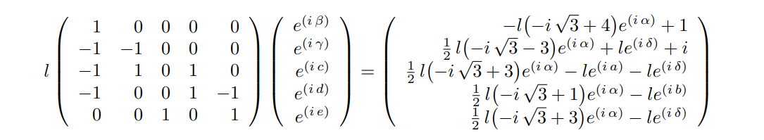
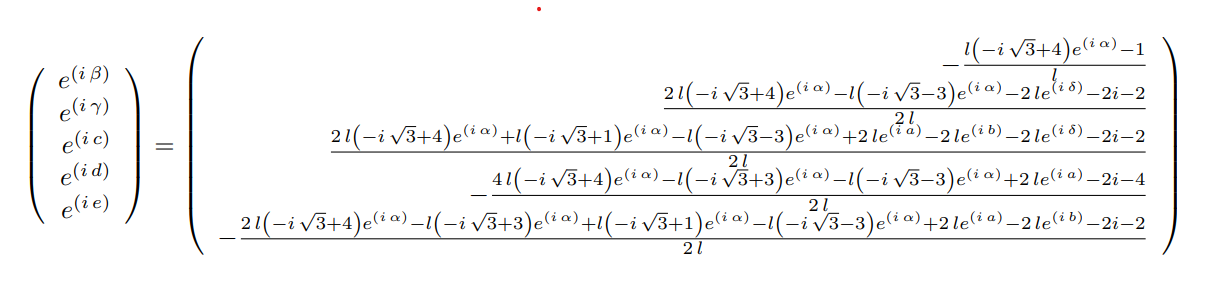
We are now considering a system with one distance variable $l$, and 10 angle variables $\alpha$, $\beta$, $\gamma$, $\delta$, $\rho$, $a$, $b$, $c$, $d$ and $e$. The said trigonometric system of equations is consistuted of 11 equations as described below:
$$ 0 = l \left( {4} \cos{\left({{\alpha}}\right)} + \cos{\left({{\alpha} - \frac{{\pi}}{{3}}}\right)} + \cos{\left({{\beta}}\right)} + \cos{\left({{\alpha} - \frac{{2} {\pi}}{{3}}}\right)} \right) - {1} $$ $$ 0 = {4} \sin{\left({{\alpha}}\right)} + \sin{\left({{\alpha} - \frac{{\pi}}{{3}}}\right)} + \sin{\left({{\beta}}\right)} + \sin{\left({{\alpha} - \frac{{2} {\pi}}{{3}}}\right)} $$ $$ 0 = {2} \cos{\left({{\alpha}}\right)} - \cos{\left({{\gamma}}\right)} - \cos{\left({{\delta}}\right)} - \cos{\left({{\rho}}\right)} + \cos{\left({{\alpha} + \frac{{2} {\pi}}{{3}}}\right)} $$ $$ 0 = l \left( {2} \sin{\left({{\alpha}}\right)} - \sin{\left({{\gamma}}\right)} - \sin{\left({{\delta}}\right)} - \sin{\left({{\rho}}\right)} + \sin{\left({{\alpha} + \frac{{2} {\pi}}{{3}}}\right)} \right) - {1} $$ $$ 0 = \cos{\left({a}\right)} - \cos{\left({b}\right)} - \cos{\left({c}\right)} + \cos{\left({{\gamma}}\right)} + \cos{\left({{\alpha} - \frac{{\pi}}{{3}}}\right)} $$ $$ 0 = \sin{\left({a}\right)} - \sin{\left({b}\right)} - \sin{\left({c}\right)} + \sin{\left({{\gamma}}\right)} + \sin{\left({{\alpha} - \frac{{\pi}}{{3}}}\right)} $$ $$ 0 = \cos{\left({c}\right)} + \cos{\left({e}\right)} - \cos{\left({{\alpha} - \frac{{\pi}}{{3}}}\right)} - \cos{\left({{\alpha}}\right)} + \cos{\left({{\delta}}\right)} $$ $$ 0 = \sin{\left({c}\right)} + \sin{\left({e}\right)} - \sin{\left({{\alpha} - \frac{{\pi}}{{3}}}\right)} - \sin{\left({{\alpha}}\right)} + \sin{\left({{\delta}}\right)} $$ $$ 0 = \cos{\left({b}\right)} + \cos{\left({d}\right)} - \cos{\left({{\rho}}\right)} - \cos{\left({{\alpha} - \frac{{\pi}}{{3}}}\right)} - \cos{\left({e}\right)} $$ $$ 0 = \sin{\left({b}\right)} + \sin{\left({d}\right)} - \sin{\left({{\rho}}\right)} - \sin{\left({{\alpha} - \frac{{\pi}}{{3}}}\right)} - \sin{\left({e}\right)} $$ $$ 0 = \cos{\left({{\rho}}\right)} + \cos{\left({{\alpha} - \frac{{\pi}}{{3}}}\right)} + \cos{\left({{\alpha}}\right)} - \cos{\left({{\gamma}}\right)} - \cos{\left({{\delta}}\right)} - \cos{\left({d}\right)} - \cos{\left({a}\right)} $$
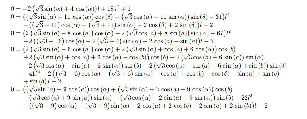
as usual, we are interested in finding the minimal polynomial of the root $l$ between 0 and 1 for which a numerical appriximation is $l \approx 0.2226926944766917$.
Below is my (unsuccessfull) attempt to use to solve this problem:
#numerical values
l = 0.2226926944766917
alpha = 0.6331728275782392
beta = -1.3273875824789818
gamma = -1.4524093897328
delta = -1.226349124695996
rho = -1.3273875824743633
a = 0.9747473834353503
b = -0.9033592481852397
c = 0.2194297013449713
d = 0.33163441038029523
e = 1.1505721363111867

# conversion to non trig variables

c0 = cos(alpha)
s0 = sin(alpha)
c1 = cos(beta)
s1 = sin(beta)
c2 = cos(gamma)
s2 = sin(gamma)
c3 = cos(delta)
s3 = sin(delta)
c4 = cos(rho)
s4 = sin(rho)
c5 = cos(a)
s5 = sin(a)
c6 = cos(b)
s6 = sin(b)
c7 = cos(c)
s7 = sin(c)
c8 = cos(d)
s8 = sin(d)
c9 = cos(e)
s9 = sin(e)

# system of equations
eq1 = 4*c0+(c0+sqrt(3)*s0)/2+c1+(-c0+sqrt(3)*s0)/2-1/l
eq2 = 4*s0+(-sqrt(3)*c0+s0)/2+s1+(-sqrt(3)*c0-s0)/2
eq3 = 2*c0-c2-c3-c4-(c0+sqrt(3)*s0)/2
eq4 = 2*s0-s2-s3-s4+(sqrt(3)*c0-s0)/2-1/l
eq5 = c5-c6-c7+c2+(c0+sqrt(3)*s0)/2
eq6 = s5-s6-s7+s2+(-sqrt(3)*c0+s0)/2
eq7 = c7+c9-(c0+sqrt(3)*s0)/2-c0+c3
eq8 = s7+s9-(-sqrt(3)*c0+s0)/2-s0+s3
eq9  = c6+c8-c4-(c0+sqrt(3)*s0)/2-c9
eq10 = s6+s8-s4-(-sqrt(3)*c0+s0)/2-s9
eq11 = c4+(c0+sqrt(3)*s0)/2+c0-c2-c3-c8-c5


#numerical check
show(eq1.numerical_approx())
show(eq2.numerical_approx())
show(eq3.numerical_approx())
show(eq4.numerical_approx())
show(eq5.numerical_approx())
show(eq6.numerical_approx())
show(eq7.numerical_approx())
show(eq8.numerical_approx())
show(eq9.numerical_approx())
show(eq10.numerical_approx())
show(eq11.numerical_approx())


reset()
from time import time as stime
RR.<l, c0, c1, c2, c3, c4, c5, c6, c7, c8, c9, s0, s1, s2, s3, s4, s5, s6, s7, s8, s9, str3 >=AA[]
Sys = [ # linear equations
    l*(4*c0+(c0+str3*s0)/2+c1+(-c0+str3*s0)/2)-1,
    4*s0+(-str3*c0+s0)/2+s1+(-str3*c0-s0)/2,
    2*c0-c2-c3-c4-(c0+str3*s0)/2,
    l*(2*s0-s2-s3-s4+(str3*c0-s0)/2)-1,
    c5-c6-c7+c2+(c0+str3*s0)/2,
    s5-s6-s7+s2+(-str3*c0+s0)/2,
    c7+c9-(c0+str3*s0)/2-c0+c3,
    s7+s9-(-str3*c0+s0)/2-s0+s3,
    c6+c8-c4-(c0+str3*s0)/2-c9,
    s6+s8-s4-(-str3*c0+s0)/2-s9,
    c4+(c0+str3*s0)/2+c0-c2-c3-c8-c5,
    # Trigonometrics
    str3^2-3,
    s0^2 + c0^2 -1,
    s1^2 + c1^2 -1,
    s2^2 + c2^2 -1,
    s3^2 + c3^2 -1,
    s4^2 + c4^2 -1,
    s5^2 + c5^2 -1,
    s6^2 + c6^2 -1,
    s7^2 + c7^2 -1,
    s8^2 + c8^2 -1,
    s9^2 + c9^2 -1]
J1 = RR.ideal(Sys)
print("Solution dimension = ", J1.dimension())
t0 = stime()
Sols = J1.variety()
t1 = stime()
print("Number of solutions = ", len(Sols), ", found in %f6.3 seconds."%(t1-t0))
Errs = [abs(s[l]-0.22269269447669) for s in Sols]
Sol = Sols[Errs.index(min(Errs))]
show(Sols)
t2 = stime()
print(Sol[r])
P = Sol[l].minpoly()
t3 = stime()
print("Minimal polynomial (found in %f6.3 seconds) :"%(t3-t2))
print(P)
Permalink for testing purposes:
https://sagecell.sagemath.org/?z=eJx9...
Additionnal Permalink using Elimination_ideal, also fails:
https://sagecell.sagemath.org/?z=eJy1...
In this case sagemathcell websocket kernell crashes at the following line J1 = RR.ideal(Sys). Because no error message is returned we have no idea what is going wrong. It could yet again be a mistake on our side. We have included all numerical checks of the system's equations in order to facilitate further analysis. We are aware that this particular system is now much larger than the ones in previous posts, but do not know if it does not work because of a mistake on our side, or if we are pushing beyond the limits of sagemath?
In advance, thanks for your help.
kr,

J1 = RR.ideal(Sys)works fine at Sagecell. Perhaps, it's time to update your local Sage.Oh ok but, actually I do not have a local Sage installation. I am using the online version on https://sagecell.sagemath.org/ ...
I do not see the crash at Sagecell.
Here is what I see in the browser network console
No results returned .
Permalink added in the Question Edit Box under the Sage Code Box
I used you link. Sagecell goes into long computation of dimension, but the ideal is constructed without an issue. No crash.
I also used this link. It starts well, prints the nuerical values of the quantities defining the problem, displaying a rotating image signalling a computation in progress. Then, after about two minutes, the rotating image disappears.
Crash ?
2 minutes is about the time limit for Sagecell. I would not assume a crash but just a timeout. At very least,
J1 = RR.ideal(Sys)works fine, which can be seen via adding aprintstatement after it.I don't understand. There is a print statement right after that
print("Solution dimension = ", J1.dimension()), however it never prints anything. Why ? ifJ1 = RR.ideal(Sys)works fine why does the rest of the programm not execute afterwards?Indeed SageMathCell has a time limit for computations. That print statement is not executed because
J1.dimension()is a big (Groebner basis) computation that exceeds the timeout. I am running (a slight modification of) your script on a supercomputer with a 7 day time limit. You could also try alternatives like usingmsolve.Wow !! That is remarkable ... Thank you so much for your help. Thanks for the explanations. Hopefully 7 days will be enough. fingers crossed
msolveis supported from within Sage, btw.Thanks a lot! I will have a look at it.
@rburing: Computing variety over
AAhere is an overkill and is inefficient. It may be more feasible to compute the elimination ideal overQuadraticField(3)as explained in the linked question.We undertake to solve a system involving 21 indeterminates, which is a lot given the combinatorial explosion of the Gr¨bner basis computation. We can reduce this to 11 indeterminates by using the half-angles formulas. if
Eqsis the list of the original equations, a new systemSysof equations can be obtained by :I'll look at this one.
For what it's worth, short temporary link to the code creating the ideal (the permalink is too long to fit in a comment).
J2.dimension()has already run for one hour without returning. I'm not optimistic...I threw the towel after 7 hours waiting for
J2.dimension()to return...One needs not the dimension but rather the elimination ideal with respect to all but
lvariables. From its generators one can easily get the minimal polynomial the OP asks for.@max Alkseyev, I removed the dimension call and confirm that RR.ideal returns successfully. However, elimination_ideal does not return either (see additionnal Permalink in the question Box).
@aobara: It's also worth to replace:
with
Thanks, I just tried but for this particular problem does not seem to be sufficient. Thanks though for the tip...