Large System of Quadratic Trigonometric Equations
Following the answers provided in 2 previous posts https://ask.sagemath.org/question/706... and https://ask.sagemath.org/question/726..., we tried to apply the proposed methods to a yet more complex system of trigonometric equations.
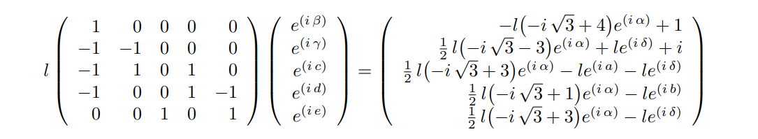
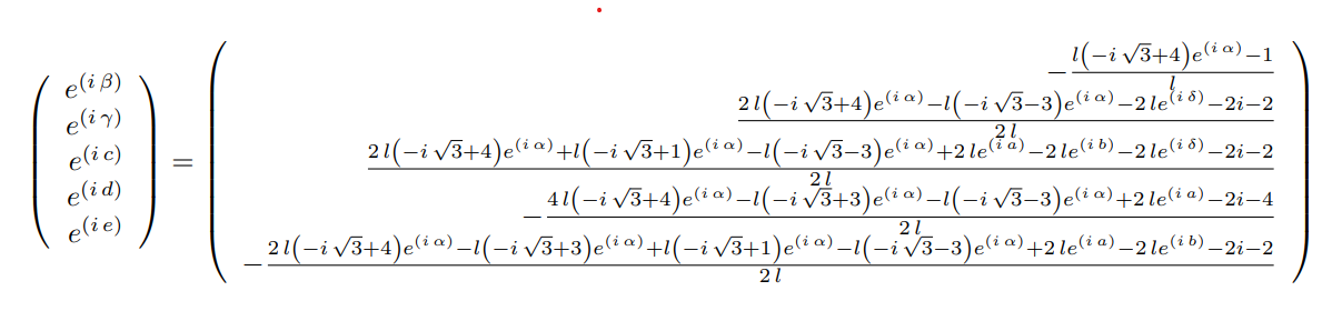
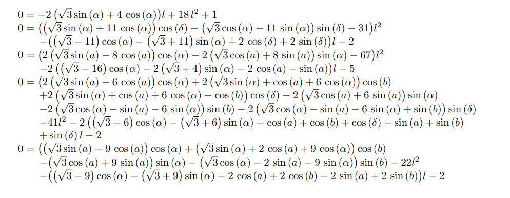
We are now considering a system with one distance variable $l$, and 10 angle variables $\alpha$, $\beta$, $\gamma$, $\delta$, $\rho$, $a$, $b$, $c$, $d$ and $e$. The said trigonometric system of equations is consistuted of 11 equations as described below:
$$ 0 = l \left( {4} \cos{\left({{\alpha}}\right)} + \cos{\left({{\alpha} - \frac{{\pi}}{{3}}}\right)} + \cos{\left({{\beta}}\right)} + \cos{\left({{\alpha} - \frac{{2} {\pi}}{{3}}}\right)} \right) - {1} $$ $$ 0 = {4} \sin{\left({{\alpha}}\right)} + \sin{\left({{\alpha} - \frac{{\pi}}{{3}}}\right)} + \sin{\left({{\beta}}\right)} + \sin{\left({{\alpha} - \frac{{2} {\pi}}{{3}}}\right)} $$ $$ 0 = {2} \cos{\left({{\alpha}}\right)} - \cos{\left({{\gamma}}\right)} - \cos{\left({{\delta}}\right)} - \cos{\left({{\rho}}\right)} + \cos{\left({{\alpha} + \frac{{2} {\pi}}{{3}}}\right)} $$ $$ 0 = l \left( {2} \sin{\left({{\alpha}}\right)} - \sin{\left({{\gamma}}\right)} - \sin{\left({{\delta}}\right)} - \sin{\left({{\rho}}\right)} + \sin{\left({{\alpha} + \frac{{2} {\pi}}{{3}}}\right)} \right) - {1} $$ $$ 0 = \cos{\left({a}\right)} - \cos{\left({b}\right)} - \cos{\left({c}\right)} + \cos{\left({{\gamma}}\right)} + \cos{\left({{\alpha} - \frac{{\pi}}{{3}}}\right)} $$ $$ 0 = \sin{\left({a}\right)} - \sin{\left({b}\right)} - \sin{\left({c}\right)} + \sin{\left({{\gamma}}\right)} + \sin{\left({{\alpha} - \frac{{\pi}}{{3}}}\right)} $$ $$ 0 = \cos{\left({c}\right)} + \cos{\left({e}\right)} - \cos{\left({{\alpha} - \frac{{\pi}}{{3}}}\right)} - \cos{\left({{\alpha}}\right)} + \cos{\left({{\delta}}\right)} $$ $$ 0 = \sin{\left({c}\right)} + \sin{\left({e}\right)} - \sin{\left({{\alpha} - \frac{{\pi}}{{3}}}\right)} - \sin{\left({{\alpha}}\right)} + \sin{\left({{\delta}}\right)} $$ $$ 0 = \cos{\left({b}\right)} + \cos{\left({d}\right)} - \cos{\left({{\rho}}\right)} - \cos{\left({{\alpha} - \frac{{\pi}}{{3}}}\right)} - \cos{\left({e}\right)} $$ $$ 0 = \sin{\left({b}\right)} + \sin{\left({d}\right)} - \sin{\left({{\rho}}\right)} - \sin{\left({{\alpha} - \frac{{\pi}}{{3}}}\right)} - \sin{\left({e}\right)} $$ $$ 0 = \cos{\left({{\rho}}\right)} + \cos{\left({{\alpha} - \frac{{\pi}}{{3}}}\right)} + \cos{\left({{\alpha}}\right)} - \cos{\left({{\gamma}}\right)} - \cos{\left({{\delta}}\right)} - \cos{\left({d}\right)} - \cos{\left({a}\right)} $$
as usual, we are interested in finding the minimal polynomial of the root $l$ between 0 and 1 for which a numerical appriximation is $l \approx 0.2226926944766917$.
Below is my (unsuccessfull) attempt to use to solve this problem:
#numerical values
l = 0.2226926944766917
alpha = 0.6331728275782392
beta = -1.3273875824789818
gamma = -1.4524093897328
delta = -1.226349124695996
rho = -1.3273875824743633
a = 0.9747473834353503
b = -0.9033592481852397
c = 0.2194297013449713
d = 0.33163441038029523
e = 1.1505721363111867

# conversion to non trig variables

c0 = cos(alpha)
s0 = sin(alpha)
c1 = cos(beta)
s1 = sin(beta)
c2 = cos(gamma)
s2 = sin(gamma)
c3 = cos(delta)
s3 = sin(delta)
c4 = cos(rho)
s4 = sin(rho)
c5 = cos(a)
s5 = sin(a)
c6 = cos(b)
s6 = sin(b)
c7 = cos(c)
s7 = sin(c)
c8 = cos(d)
s8 = sin(d)
c9 = cos(e)
s9 = sin(e)

# system of equations
eq1 = 4*c0+(c0+sqrt(3)*s0)/2+c1+(-c0+sqrt(3)*s0)/2-1/l
eq2 = 4*s0+(-sqrt(3)*c0+s0)/2+s1+(-sqrt(3)*c0-s0)/2
eq3 = 2*c0-c2-c3-c4-(c0+sqrt(3)*s0)/2
eq4 = 2*s0-s2-s3-s4+(sqrt(3)*c0-s0)/2-1/l
eq5 = c5-c6-c7+c2+(c0+sqrt(3)*s0)/2
eq6 = s5-s6-s7+s2+(-sqrt(3)*c0+s0)/2
eq7 = c7+c9-(c0+sqrt(3)*s0)/2-c0+c3
eq8 = s7+s9-(-sqrt(3)*c0+s0)/2-s0+s3
eq9  = c6+c8-c4-(c0+sqrt(3)*s0)/2-c9
eq10 = s6+s8-s4-(-sqrt(3)*c0+s0)/2-s9
eq11 = c4+(c0+sqrt(3)*s0)/2+c0-c2-c3-c8-c5


#numerical check
show(eq1.numerical_approx())
show(eq2.numerical_approx())
show(eq3.numerical_approx())
show(eq4.numerical_approx())
show(eq5.numerical_approx())
show(eq6.numerical_approx())
show(eq7.numerical_approx())
show(eq8.numerical_approx())
show(eq9.numerical_approx())
show(eq10.numerical_approx())
show(eq11.numerical_approx())


reset()
from time import time as stime
RR.<l, c0, c1, c2, c3, c4, c5, c6, c7, c8, c9, s0, s1, s2, s3, s4, s5, s6, s7, s8, s9, str3 >=AA[]
Sys = [ # linear equations
    l*(4*c0+(c0+str3*s0)/2+c1+(-c0+str3*s0)/2)-1,
    4*s0+(-str3*c0+s0)/2+s1+(-str3*c0-s0)/2,
    2*c0-c2-c3-c4-(c0+str3*s0)/2,
    l*(2*s0-s2-s3-s4+(str3*c0-s0)/2)-1,
    c5-c6-c7+c2+(c0+str3*s0)/2,
    s5-s6-s7+s2+(-str3*c0+s0)/2,
    c7+c9-(c0+str3*s0)/2-c0+c3,
    s7+s9-(-str3*c0+s0)/2-s0+s3,
    c6+c8-c4-(c0+str3*s0)/2-c9,
    s6+s8-s4-(-str3*c0+s0)/2-s9,
    c4+(c0+str3*s0)/2+c0-c2-c3-c8-c5,
    # Trigonometrics
    str3^2-3,
    s0^2 + c0^2 -1,
    s1^2 + c1^2 -1,
    s2^2 + c2^2 -1,
    s3^2 + c3^2 -1,
    s4^2 + c4^2 -1,
    s5^2 + c5^2 -1,
    s6^2 + c6^2 -1,
    s7^2 + c7^2 -1,
    s8^2 + c8^2 -1,
    s9^2 + c9^2 -1]
J1 = RR.ideal(Sys)
print("Solution dimension = ", J1.dimension())
t0 = stime()
Sols = J1.variety()
t1 = stime()
print("Number of solutions = ", len(Sols), ", found in %f6.3 seconds."%(t1-t0))
Errs = [abs(s[l]-0.22269269447669) for s in Sols]
Sol = Sols[Errs.index(min(Errs))]
show(Sols)
t2 = stime()
print(Sol[r])
P = Sol[l].minpoly()
t3 = stime()
print("Minimal polynomial (found in %f6.3 seconds) :"%(t3-t2))
print(P)
Permalink for testing purposes:
https://sagecell.sagemath.org/?z=eJx9...
Additionnal Permalink using Elimination_ideal, also fails:
https://sagecell.sagemath.org/?z=eJy1...
In this case sagemathcell websocket kernell crashes at the following line J1 = RR.ideal(Sys). Because no error message is returned we have no idea what is going wrong. It could yet again be a mistake on our side. We have included all numerical checks of the system's equations in order to facilitate further analysis. We are aware that this particular system is now much larger than the ones in previous posts, but do not know if it does not work because of a mistake on our side, or if we are pushing beyond the limits of sagemath?
In advance, thanks for your help.
kr,

J1 = RR.ideal(Sys)works fine at Sagecell. Perhaps, it's time to update your local Sage.Oh ok but, actually I do not have a local Sage installation. I am using the online version on https://sagecell.sagemath.org/ ...
I do not see the crash at Sagecell.
Here is what I see in the browser network console
No results returned .
Permalink added in the Question Edit Box under the Sage Code Box