Select component of an `implicit_plot` curve
I'd like to plot one of the connected components of a plot. This is like
sage: x, y = SR.var('x, y', domain='real')
sage: F0 = x^2 - y^2 - 1
sage: B0 = 3.5
sage: G0 = implicit_plot(F0, (x, -B0, B0), (y, -B0, B0), gridlines=True)
sage: G0.show(figsize=5)
Launched png viewer for Graphics object consisting of 1 graphics primitive
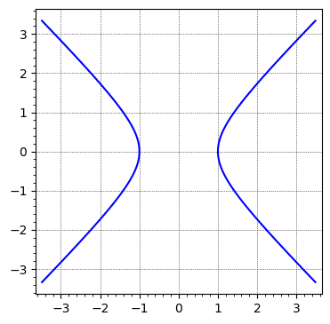
which one could solve and manually select the connected components. In my case, I deal with an equation that is inconvenient to plot directly from the solution. Is there a command or a feature to `implicit plot' which has the effect of "taking this connected component of the solution" (e.g. in the example, passing through $(-1,0)$?) Also I wouldn't like to restrict to either positive or negative $x$ (my curve is somehow more complicated and restricting to regions doesn't work).
I excluded the curve to make this a minimal example, but it's probably helpful to know that I don't know how to easily parametrize it. Is something like
   sage: F = -1/720*x^6*y*cos(sqrt(2)*pi) + 1/144*x^4*y^3*cos(sqrt(2)*pi) - 1/240*x^2*y^5*cos(sqrt(2)*pi)+ 1/5040*y^7*cos(sqrt(2)*pi) - 1/5040*x^7*sin(sqrt(2)*pi) + 1/240*x^5*y^2*sin(sqrt(2)*pi) -1/144*x^3*y^4*sin(sqrt(2)*pi) + 1/720*x*y^6*sin(sqrt(2)*pi) +1/114688*720^(2/5)*abs(-2*sqrt(5) + 10)^(7/2)*cos(2/5*sqrt(2)*pi)*cos(7/2*arctan2(0, -2*sqrt(5) + 10))   + 1/114688*720^(2/5)*abs(-2*sqrt(5) + 10)^(7/2)*sin(2/5*sqrt(2)*pi)*sin(7/2*arctan2(0, -2*sqrt(5) + 10))- 3/8192*720^(2/5)*sqrt(5)*abs(-2*sqrt(5) + 10)^(5/2)*cos(2/5*sqrt(2)*pi)*cos(5/2*arctan2(0,  -2*sqrt(5) + 10)) - 3/8192*720^(2/5)*sqrt(5)*abs(-2*sqrt(5) + 10)^(5/2)*sin(2/5*sqrt(2)*pi)   *sin(5/2*arctan2(0, -2*sqrt(5) + 10)) - 9/8192*720^(2/5)*abs(-2*sqrt(5) + 10)^(5/2)   *cos(2/5*sqrt(2)*pi)*cos(5/2*arctan2(0, -2*sqrt(5) + 10)) - 9/8192*720^(2/5)*abs(-2*sqrt(5)  + 10)^(5/2)*sin(2/5*sqrt(2)*pi)*sin(5/2*arctan2(0, -2*sqrt(5) + 10))+ 15/2048*720^(2/5)*sqrt(5)*abs(-2*sqrt(5) + 10)^(3/2)*cos(2/5*sqrt(2)*pi)*cos(3/2*arctan2(0,   -2*sqrt(5) + 10)) + 15/2048*720^(2/5)*sqrt(5)*abs(-2*sqrt(5)  + 10)^(3/2)*sin(2/5*sqrt(2)*pi)*sin(3/2*arctan2(0, -2*sqrt(5) + 10))  + 35/2048*720^(2/5)*abs(-2*sqrt(5) + 10)^(3/2)*cos(2/5*sqrt(2)*pi)*cos(3/2*arctan2(0, -2*sqrt(5) + 10)) + 35/2048*720^(2/5)*abs(-2*sqrt(5) + 10)^(3/2)*sin(2/5*sqrt(2)*pi)*sin(3/2*arctan2(0, -2*sqrt(5)  + 10)) - 5/64*720^(2/5)*sqrt(5)*sqrt(abs(-2*sqrt(5)  + 10))*cos(2/5*sqrt(2)*pi)*cos(1/2*arctan2(0, -2*sqrt(5) + 10))  - 5/64*720^(2/5)*sqrt(5)*sqrt(abs(-2*sqrt(5) + 10))*sin(2/5*sqrt(2)*pi)*sin(1/2*arctan2(0, -2*sqrt(5) + 10)) - 25/256*720^(2/5)*sqrt(abs(-2*sqrt(5) + 10))*cos(2/5*sqrt(2)*pi)*cos(1/2*arctan2(0, -2*sqrt(5)  + 10)) - 25/256*720^(2/5)*sqrt(abs(-2*sqrt(5) + 10))*sin(2/5*sqrt(2)*pi)*sin(1/2*arctan2(0, -2*sqrt(5)  + 10)) + x*y + 5/56*720^(2/5)*sqrt(5)*sin(2/5*sqrt(2)*pi) - 5/56*720^(2/5)*sin(2/5*sqrt(2)*pi)
sage: B = 7.5
sage: G = implicit_plot(F, (x, -B, B), (y, -B, B), gridlines=True)
sage: G.show(figsize=5)
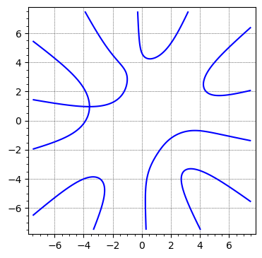
This has many connected components (on the finite plane), the square root of two is just to match another conventions, you could ignore this and any number-theoretical stuff, just think about the sort of not low degree polynomial in two variables. Cannot upload the plot yet.

To make it more answerable: what is your more complicated equation?
@rburing Hi, thanks, I added it.
After staring at the complicated equation for some time, here is a more concise rephrasing of it.
Putting $z = x + i \, y$, there are some real constants $A$, $B$, $C$ such that the equation amounts to: $$ \operatorname{Re}\left(e^{i \, A} \frac{z^7}{7!} + e^{i \, B} \frac{z^2}{2!}\right) = C $$
The degree 7 explains the 7 components of the curve.
The approach in @FrédéricC's answer to Ask Sage question 54765 might give inspiration here.
@slelievre Hi, thanks for the insight and suggestions (and the edit!)