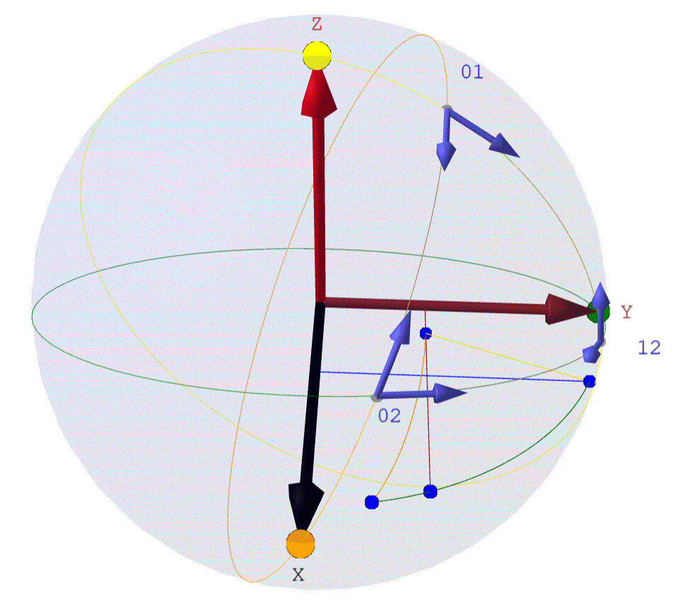
integral of function with sgn (x,I) inside

asked 2021-01-23 09:19:33 +0100

ortollj
1341 ●23 ●63 ●96

updated 2021-01-23 09:26:21 +0100

I encounter a problem on an integral calculation, and I do not know how to find a workaround. (I mean a mathematically correct workaround, not the questionable tinkering of replacing SGN (f (x, I)) by -1 !!! that I did to get a numeric value ;-) ). if I comment out lines (77,78) and (128,129) I get an error:

ValueError: The function to be integrated depends on 2 variables (x, z), and so cannot be integrated in one dimension. Please fix additional variables with the 'params' argument

Does somebody knows what 'params' I must set in function numerical_integral ? code on sagecell

show("###########################################################") 
show("Compute Surface of the spherical triangle and XY plan") 
show("###########################################################") 
var('x,y')
rNum=1

var('xLow,xUp,yLow,yUp')

# rounding values
PtsL=       [[0.13795, 0.37902], [0.33554, 0.92189], [0.84803, 0.2028], [0.80141, 0.37902]]
PtsNamesL = [      'xy01',            'xy12',              'xy02',          'xyCut']

ellipse0 = 1/2*sqrt(-x^2 + 1)*sqrt(-sqrt(2) + 2)
ellipse1 = x*cos(1/9*pi)/sin(1/9*pi)
ellipse2 = sqrt(-4/3*x^2 + 1)

plt = list_plot(PtsL, color='blue', size=30)
pt_opt = {'color': 'blue', 'horizontal_alignment': 'left', 'vertical_alignment': 'bottom'}
plt += sum(text(name, vector(pt), **pt_opt) for name, pt in zip(PtsNamesL, PtsL))
plt += line([[0, PtsL[3][1]], PtsL[3]], color='brown', thickness=2, linestyle='dashed')
plt += line([[PtsL[1][0], 0], PtsL[1]], color='blue', thickness=2, linestyle='dashed')
plt+=implicit_plot(ellipse0-y,(x,0,1),(y,0,1),color='orange')
plt+=plot(ellipse1,(x,0.1,PtsL[1][0]),color='yellow')
plt+=implicit_plot(ellipse2-y,(x,0,1),(y,0,1),color='green')



rS(x,y,z)=(x,y,sqrt(rNum^2-x^2-y^2))
rSdx=diff(rS,x,1)
rSdy=diff(rS,y,1)
assume(0<x<1)
assume(0<y<1)
assume(rNum^2-x^2-y^2 >0)

show("r diff x : ",rSdx," \t r diff y : ",rSdy)
rSds=(vector(rSdx).cross_product(vector(rSdy)))
# I don't use rSds.norm(),because it is adding abs function
# because for us R^2-x^2-y^2 >=0 
dsNorm=sqrt(rSds[0]^2+rSds[1]^2+rSds[2]^2)
show("ds : ",rSds," \t norm : ",dsNorm)

show("order of integration, Y,X : FIRST part, left side of the blue line ")

Pxy0 = plt
Pxy0+= plot([ellipse0, ellipse1], (PtsL[0][0], PtsL[1][0]), fill={0: [1]}, fillcolor='#ccc', fillalpha=.3)
Pxy0+=implicit_plot(ellipse0-y,(x,0,1),(y,0,1),color='orange')
Pxy0+=plot(ellipse1,(x,(PtsL[0][0]),(PtsL[1][0])),color='yellow')
Pxy0+=implicit_plot(ellipse2-y,(x,0,1),(y,0,1),color='green')
Pxy0.show(xmin=0, xmax=1, ymin=0, ymax=1, aspect_ratio=1, figsize=8)

show("first piece delimited by yellow curve ,orange curve and blue line in xy plan")

eqLimitL=[]


eqLimitL.append(yLow==ellipse0)
eqLimitL.append(yUp==ellipse1)

eqLimitL.append(xLow==PtsL[0][0])
eqLimitL.append(xUp==PtsL[1][0])


arrondi=10
# spherical triangle partaged in two pieces
# first piece delimited by yellow curve ,orange curve and blue line in xy plan
show(LatexExpr(r"\text{surface of first piece of spherical Triangle} \,=\,"
+r"\int_{"+latex(eqLimitL[0])+"}^{"+latex(eqLimitL[1])+"} " \
+r"\int_{xLow="+latex(round(eqLimitL[2].rhs(),arrondi))+"}^{xUp="+latex(round(eqLimitL[3].rhs(),arrondi))+"} " \
#+r", "+latex(rS[2])+latex(dsNorm)+r" \, \, dy \, dx"))
+r", "+latex(dsNorm)+r" \, \, dy \, dx"))

intY0=(integrate(dsNorm,y,eqLimitL[0].rhs(),eqLimitL[1].rhs(),algorithm="giac"))
print(intY0)

intY00=intY0
#show(" below we replace sgn function by fsgn(x)=-1 because numerical_integral can't integrate with sgn ")
fsgn(x)= -1
intY00=intY0.substitute_function(sgn,fsgn)

show("intY0 with sgn Function: ", intY0)
show("intY00 subs of sgn: ", intY00)
intYX00=numerical_integral(intY00,eqLimitL[2].rhs(),eqLimitL[3].rhs())
show("First spherical surface  piece after numerical integration : ", intYX00)



var('xLow,xUp,yLow,yUp',domain='real')
show("order of integration, Y,X : Second part, rigth side of the blue line ") 

Pxy1 = plt
Pxy1+= plot([ellipse0, ellipse2], (PtsL[1][0], PtsL[2][0]), fill={0: [1]}, fillcolor='#ccc', fillalpha=.3)
Pxy1+= plot([ellipse0, ellipse2], (PtsL[1][0], PtsL[2][0]), fill={0: [1]}, fillcolor='#ccc', fillalpha=.3)
Pxy1+=implicit_plot(ellipse0-y,(x,0,1),(y,0,1),color='orange')
Pxy1+=plot(ellipse1,(x,PtsL[0][0],PtsL[1][0]),color='yellow')
Pxy1+=implicit_plot(ellipse2-y,(x,0,1),(y,0,1),color='green')
Pxy1.show(xmin=0, xmax=1, ymin=0, ymax=1, aspect_ratio=1, figsize=8)



eqLimitL=[]
# delimited y area
#assume(PtsL[2][1]<=ellipse0 <=PtsL[1][1])
#assume(PtsL[2][1]<=ellipse2 <=PtsL[1][1])
# delimited x area
eqLimitL.append(yLow==ellipse0)
eqLimitL.append(yUp==ellipse2)

eqLimitL.append(xLow==PtsL[1][0])
eqLimitL.append(xUp==PtsL[2][0])


arrondi=10
# spherical triangle partaged in two pieces
# Second piece delimited by blue line ,orange curve and green curve in xy plan
show(LatexExpr(r"\text{surface of second piece of spherical Triangle} \,=\,"
+r"\int_{"+latex(eqLimitL[0])+"}^{"+latex(eqLimitL[1])+"} " \
+r"\int_{xLow="+latex(round(eqLimitL[2].rhs(),arrondi))+"}^{xUp="+latex(round(eqLimitL[3].rhs(),arrondi))+"} " \
#+r", "+latex(rS[2])+latex(dsNorm)+r" \, \, dy \, dx"))
+r", "+latex(dsNorm)+r" \, \, dy \, dx"))

#intY1=(integrate(dsNorm,y,eqLimitL[0].rhs(),eqLimitL[1].rhs(),algorithm="giac"))
intY1=(integrate(dsNorm,y,yLow,yUp,algorithm="giac"))
print(intY1)
intY11=intY1.subs(eqLimitL)
show("intY1 : ",intY11)
intY111=intY11
#show(" below we replace sgn function by fsgn(x)=-1 because numerical_integral can't integrate with sgn ")
fsgn(x)= -1
intY111=intY11.substitute_function(sgn,fsgn)


show("intY11 with sgn Function: ", intY11)
show("intY111 subs of sgn: ", intY111)
intYX111=numerical_integral(intY111,eqLimitL[2].rhs().n(),eqLimitL[3].rhs().n())
show("Second spherical surface piece after numerical integration : ", intYX111)
show("total Triangle area Computed by surface integration: ", intYX00[0]+intYX111[0])
#show('Total TriAngle Area Computed with Harriot Theorem : ',HarriotArea,' \t with R = ',rNum)
#show(" We can also verify the computation in multiplying the radius by 2(rNum at top of the file)")
#show(" and check that the surface is multiplied by 2^2=4 and the volume by 2^3=8")
#show(" you can also check the computation by changing the spherical surface with the condition,")
#show(" that this surface should be contained in first octant ")

sphere 3D

Comments

I forgot to tell: do not reset the file in notebook, it will crash the notebook

ortollj ( 2021-01-23 10:27:22 +0100 )edit

I am wondering about this question.

No one answered, I know there is no obligation to answer a question, and I do not claim an answer, moreover maybe that my mathematical question is not relevant. and therefore I am wondering about my question, I would have liked an opinion . (One can tick several boxes)

1)I messed up in my integral calculation

2) my question is scatty kind of: https://ask.sagemath.org/question/553... (maybe a troll behind this question ? not sure )

3)my question is not really interesting

4)there is no simple solution to my question

ortollj ( 2021-01-24 11:31:26 +0100 )edit

I explain what I wanted to do in the entire code ,(probably naively and doomed to failure, but that's okay ;-),this is not the point ) the code above was an excerpt :

I wanted to try to obtain an algebraic length of an arc of ellipse using Harriot's theorem. step 1) verify that we find the surface area of any spherical triangle numerically located in the 1st octant, calculated by Harriot's theorem and by the surface integral dy dx ,1) dy algebraic integral, 2) dx numeric. step 2) use the algebraic surface value obtained by Harriot to attempt to find an algebraic value of the length of an arc of ellipse

I wanted to join the full code maybe it will help somebody to answer me but it is not accepted I think because the message seems too long.

ortollj ( 2021-01-24 11:33:30 +0100 )edit

(I'm a bit ashamed of this code because I don't know how to program correctly in Python code, and maybe somebody can propose me some improvement ?). in case of my question is relevant ! ;-)

ortollj ( 2021-01-24 11:33:54 +0100 )edit

I tried to put the code on Cocalc but it seems that now there is no more share button !

ortollj ( 2021-01-24 11:40:39 +0100 )edit

see more comments

answered 2021-01-25 07:45:16 +0100

dsejas
2833 ●16 ●55 ●101

Hello, @ortollj! After studying your code, I believe the problem comes from the fact that intY0 is a function of two variables---x and z, in this case, as you can see from the output your code generates. The thing is that definite_integral can integrate only one-variable functions. That is why you get the message

ValueError: The function to be integrated depends on 2 variables (x, z), and so cannot be integrated in one dimension. Please fix additional variables with the 'params' argument

What does this mean? That Sage has noticed that there are more than one variable, and you should give the remaining variables some numerical value in order to perform the numerical integral. Basically, Sage is asking you to do something like this:

intYX00 = numerical_integral(intY0,eqLimitL[2].rhs(),eqLimitL[3].rhs(), params=[0])

That specifies that this integral is to be performed on the first variable ($x$), after replacing $z=0$. In short, if you have a $n$-variable function, you need to specify $n-1$ numerical values for the $n-1$ last variables, so that numerical_integral can perform the integral using the first variable of the function. To better understand this, consider the following example:

f(x,y,z) = x^2 * y * z
numerical_integral(f, 0, 1, params=[2,3])

This is effectively equivalent to the integral $$\int_0^16x^2\;dx$$ since the variables $y$ and $z$ have been given the values $2$ and $3$, respectively.

This brings me to the following matter: why did I use params=[0] and no other value? In this particular case, the value I choose is irrelevant, since your intY0 is defined to be a function on $(x,z)$, but in reality its value only depends on $x$. This example will clarify this words:

f(x,y) = x^2
numerical_integral(f, 0, 1, params=[0])

Since I defined $f$ to be a function of $(x,y)$, I need to use the params argument to fix the value of $y$. However, since the value of $f$ does NOT depend on $y$, I can use anything that I please, even params=[y] itself. It won't make any difference. Of course, if this function were $f(x,y)=x^2y^3$, then there would be a different result for every (numerical) value I choose for $y$ (e.g., params=[2] to integrate $8x^2$). Notice that in this particular case, I can NOT use params=[y], because that would keep $f$ as a two variable function.

Now, when you make

fsgn(x) = -1
intY00 = intY0.substitute_function(sgn,fsgn)

apparently substitute_function converts intY0 into a simple expression (not a function that maps $(x,z)$, just a formula.) You can check this if you add print(intY00). You will notice the part (x,z) |--> is now missing. In particular, now intY00 is a formula whose value depends only on $x$, but not on $z$. So, when you pass it to numerical_integral, Sage assumes it is a one-variable function, and that way it is able to integrate.

I believe that answers your question. However, there are a few additional observations that could help you:

I can see that you used assume(0<x<1); I also did that. I was quite surprised to see that this had no effect on the sgn function. Indeed, here is an example that should return 1, but does not:
```
var('x', domain='real')
assume(0<x<1)
sgn(x)
```
However, that should not be a problem, since the integration algorithm will anyway evaluate the sgn function and return an adequate value.
I recommend in this case to remove the variable $z$ from the definition of your functions, since their values do not depend on that variable. That should eliminate the necessity of using the params argument to eliminate $z$, when it is not needed in the first place.
Unfortunately, in this particular case, you will still need to manually replace the value for sgn, since intY0 has this expression in it:
```
sgn(4*x^2*e^(2/9*I*pi) + e^(4/9*I*pi) - 2*e^(2/9*I*pi) + 1)
```
Sage seems unable to deal with this expression. Indeed, I get the message
```
TypeError: unable to coerce to a real number
```
However, replacing only that part with fsgn(x) or '(-1)' (leaving the other sgn) in intY0, returns the correct result without any problem. BUT BE CAREFULL: For complex numbers $z$, the signum function is defined by

$$\operatorname{sgn}(z) = \frac{z}{|z|}.$$

Unfortunately, the last bad news is that numerical_integral cannot deal with complex functions. Hopefully, there is a solution to this problem, but I can think of it right now...

I hope this answers your questions!

edit flag offensive delete link

Comments

Thanks a lot @dsejas, thousands of thank !

ortollj ( 2021-01-25 08:14:04 +0100 )edit

Happy to help!

dsejas ( 2021-01-26 08:37:15 +0100 )edit

the method given by @Juanjo .nintegral() in comments above (see more comments)does not work.

the first spherical triangle surface can't be inferior to flat first xy triangle.

triangleXY=(PtsL[1][1]-PtsL[0][1])*(PtsL[1][0]-PtsL[0][0])/2 =0.0536328416500000

ortollj ( 2021-01-27 09:53:45 +0100 )edit

add a comment

Your Answer

Please start posting anonymously - your entry will be published after you log in or create a new account.

integral of function with sgn (x,I) inside

Comments

1 Answer

Comments

Your Answer

Question Tools

Stats

integral of function with sgn (x,I) inside edit

Comments

1 Answer

Comments

Your Answer

Question Tools

Stats

integral of function with sgn (x,I) inside