Ask Your Question
0

How show vector or matrix in legend label of plot in latex?

asked 2021-01-16 14:32:42 +0200

rob gravatar image

We can insert latex in legend labels by surrounding the text with '$'. But it doesn't work for a vector (matrix, array), e.g.

\left[\begin{array}{r} 1 \\ 0 \end{array}\right]

Is there any way to display vector in latex in legend label?

edit retag flag offensive close merge delete

2 Answers

Sort by ยป oldest newest most voted
0

answered 2021-01-17 13:46:20 +0200

rob gravatar image

updated 2021-01-17 13:48:19 +0200

The following code won't work:

plot(x^2, legend_label=r'$v=\left[\begin{array}{r}1\\0\end{array}\right]$')

But if the type of parentheses doesn't matter (and for me it doesn't, I just care about the vertical vector) then the simple workaround, without having to install additional packages, is to use \binom:

plot(x^2, legend_label=r'$v=\binom{1}{1}$')

Thank you again @dsejas for inspiration to find such a solution.

edit flag offensive delete link more
3

answered 2021-01-17 04:36:13 +0200

dsejas gravatar image

Hello, @rob! One possible way to solve your problem is to override Sage's LaTeX engine and to let the formula rendering work be taken care of by your own LaTeX installation. Here is what you have to do:

from matplotlib import rc
rc('text', usetex=True)
plot(x^2, legend_label=r'$\left[\begin{array}{r}1\\0\end{array}\right]$')

Since Sage uses the Matplotlib library to create its plots, we first import the rc function, which allows us to set specific configurations, which is exactly what we do in the second line, specifying that all text in plots will be rendered using LaTeX. The third line is just the plot of the function x^2 (I picked it up randomly just for the purpose of example), and the legend label you wanted to use. This should be the result:

image description

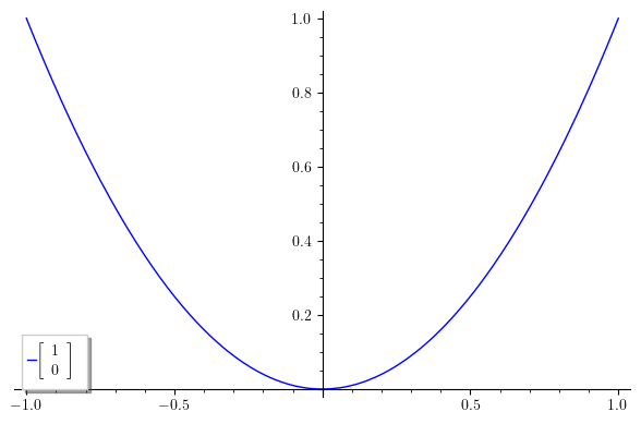
There are some downsides to this solution: First, this is not a rendering in the proper sense; what actually happens is that Matplotlib creates a LaTeX document with the code for your matrix, it compiles it on-the-fly, extracts and converts the formula to png, and finally includes the result in your plot. This leads me to the second downside: you need a LaTeX installation with the dvipng program installed, along with a couple of packages (type1cm and super-cm, if I remember correctly). As a consequence, this method doesn't work on SageCell, which has no type1ec package installed (hopefully, one day, it will be installed). However, this should work if you have a local installation of Sage and LaTeX, or you could just use CoCalc.

I would like to use the opportunity to give you a couple of suggestions. First, I am not very happy with the idea of using a matrix or vector in a legend label. Remember: scientific graphics (in particular, legend labels) are supposed to convey as much information as possible, but in the most compact and efficient way. Cluttering the plot with matrices defeats the purpose. I would suggest (if possible), using a simpler legend like just "$A$", and then using the figure caption (or the text surrounding the plot) to indicate what is $A$---for example, that is the way to go if you are writing a scientific paper. However, if you definitely require to use matrix notation, you can use the all-important transposition, writing $[1 0]^t$, or $[1 0]^T$, or $[1 0]'$, depending on your preferences on notation.

Finally, one last suggestion: SageMath (and also you in your example code) tends to use the array environment from LaTeX, and uses \left[ and \right] to produce the surrounding brackets. I recommend you to use the more modern and more carefully designed bmatrix environment (bmatrix stands for "bracketed matrix"). There are also pmatrix (parenthesized matrix), vmatrix (vertically lined matrix), etc. These environments are defined in the amsmath package, so you will need to tell Matplotlib to use it:

from matplotlib import rc
rc('text', usetex=True)
rc('text.latex', preamble=r'\usepackage{amsmath}')
plot(x^2, legend_label=r'$\begin{bmatrix}1\\0\end{bmatrix}$')

The code is self-explanatory. The result is this:

image description

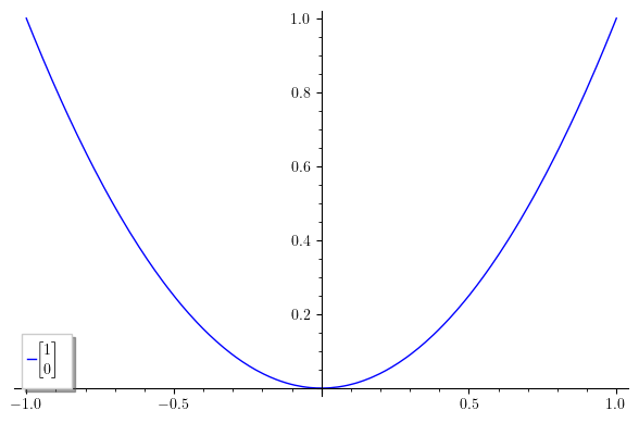
Notice the more compact and elegant matrix. Also, notice that bmatrix and its siblings don't require alignment arguments; they are fined-tuned to standard mathematical notation.

I hope this helps!

edit flag offensive delete link more

Comments

Thanks for your reply and suggestions. In CoCalc it works. Unfortunately, as you wrote in my local installation, it doesn't work (neither in jupyter nor in console). I am getting an error:

/opt/sagemath-9.2/local/lib/python3.7/site-packages/sage/repl/rich_output/display_manager.py:593: RichReprWarning: Exception in _rich_repr_ while displaying object: Failed to process string with tex because latex could not be found RichReprWarning,

But I found a very simple satisfactory workaround that requires no additional installations. (answer below)

rob gravatar imagerob ( 2021-01-17 13:20:06 +0200 )edit

As for suggestions. Unfortunately, I don't know how to upload a graphic file that visualizes my needs. The legend is to describe the coordinates of the transformed vectors presented on the plot, regardless of their showing outside the plot. Comparing horizontally written vectors is not as clear as vertical ones. And it wasn't so much about the matrix notation as it was about writing the vertical vectors. In text mode, representing the vertical vector itself was fine. But adding the vector name before it corrupts the printout.

Regarding the use of environments other than array. The horizontal separator \hline is the same as for the array environment. But how do I insert in bmatrix a (vertical) column separator used for example to represent block matrices?

rob gravatar imagerob ( 2021-01-17 13:24:56 +0200 )edit

The amsmath environments are really useful if all matrix columns are centered and no vertical separator is required. If one of these conditions is not fulfilled, then one should rely on a package like mathtools or on the standard array environment. Likewise, the space between the matrix and the delimiters can be removed with the @{} descriptor. There is a very small visual difference, if any, between, say \left(\begin{array}{@{}c@{}} 2 \\ 5 \end{array}\right) and \begin{pmatrix} 2 \\ 5 \end{pmatrix}. In a Jupyter notebook, LaTeX is rendered by MathJax, so the @{} descriptor is no recognized. In this case, the latter and \left(\begin{array}{c} 2 \\ 5 \end{array}\right) yield the same result.

Juanjo gravatar imageJuanjo ( 2021-01-17 16:56:30 +0200 )edit

Your Answer

Please start posting anonymously - your entry will be published after you log in or create a new account.

Add Answer

Question Tools

1 follower

Stats

Asked: 2021-01-16 14:32:42 +0200

Seen: 968 times

Last updated: Jan 17 '21