Filling a hyperbolic polygon

edit

Motivated by @slelievre's answer, I'm going to provide an alternative solution based on Bézier paths, which also answers this related question: Concatenate Bézier paths?

Bézier paths

Let us start by considering some facts about Bézier paths. They result from the concatenation of several linear, quadratic or cubic Bézier curves. In SageMath, Bézier paths can be obtained with the bezier_path function, as shown here:

bpath = [[(2,1),(1,0),(0,1),(1,3)], [(2,5)], [(4,9),(4,2)]]
foo = bezier_path(bpath)
show(foo, frame=True, axes=False)

The argument of bezier_path is a list of lists; except the first one, each list contains the control points and the end point of the corresponding Bézier curve, the start point being the end point of the preceding curve. This function returns a Graphics object, which wraps a BezierPath object:

sage: type(foo)
<class 'sage.plot.graphics.Graphics'>
sage: type(foo[0])
<class 'sage.plot.bezier_path.BezierPath'>

Once obtained a Bézier path, suppose that we delete the list that generated it. Can we recover such a list if we need it again? Yes, we can do it by using the vertices and codes methods defined by the BezierPath class:

sage: foo[0].vertices
array([[2., 1.],
       [1., 0.],
       [0., 1.],
       [1., 3.],
       [2., 5.],
       [4., 9.],
       [4., 2.]])
sage: foo[0].codes
[1, 4, 4, 4, 2, 3, 3]

As we can see, vertices yields a Numpy array which contains all the points involved in the generation of the Bézier path, whereas codes provides a list whose first element is always 1; the remaining elements say the order of the Bézier curve to which its associated point belongs. Please note that the first point in each curve (except the first one) is omitted. The following code allows to recover the argument of bezier_path from vertices and codes:

def recover_bpath(ver, cod):
    ii = len(cod)-1
    bpath = []
    while ii > 0:
        cc = cod[ii]
        bpath = [ ver[ii-cc+2:ii+1] ] + bpath
        ii -= cc-1
    bpath[0] = [ver[0]] + bpath[0]
    return bpath

To test this function, let us construct the list that generated foo:

sage: ver, cod = foo[0].vertices.tolist(), foo[0].codes
sage: recover_bpath(ver,cod)
[[[2.0, 1.0], [1.0, 0.0], [0.0, 1.0], [1.0, 3.0]],
 [[2.0, 5.0]],
 [[4.0, 9.0], [4.0, 2.0]]]

Here tolist serves to convert the Numpy array into a list.

It is now easy to concatenate Bézier paths, since it suffices to suitably merge their corresponding vertices and codes. We have to consider two cases, depending on whether the end point of the first path is the start point of the second path or not. This is done by the following function, whose two arguments are lists of the form [vertices, codes]:

def concatenate_bpaths(bp1, bp2, tolerance=1e-10):
    if bp1==[]: return bp2
    v1, c1 = bp1
    v2, c2 = bp2
    if norm(vector(v1[-1])-vector(v2[0]))<tolerance:
        # end point first path = start point second path
        c = c1 + c2[1:]
        v = v1 + v2[1:]
    else:
        # end point first path != start point second path
        c = c1 + [2] + c2[1:]
        v = v1 + v2
    return v, c

Note that, due to rounding errors, two points are considered equal if their distance is small enough. Let us now use these functions to graphically concatenate Bézier paths:

# Bézier paths used in this example
bp1 = [[(3,1),(1,1),(1,3),(2,4)], [(4,6)], [(5,7),(7,5)]]
bp2 = [[(7,5),(9,3),(7,2)],[(3,0),(6,-1)]]
bp3 = [[(3,0),(6,-2),(7,-1)],[(9,1),(6,1)]]
BP1 = bezier_path(bp1, color="red")
BP2 = bezier_path(bp2, color="green")
BP3 = bezier_path(bp3, color="blue")
# Vertices and codes of each Bezier path
v1, c1 = BP1[0].vertices.tolist(), BP1[0].codes
v2, c2 = BP2[0].vertices.tolist(), BP2[0].codes
v3, c3 = BP3[0].vertices.tolist(), BP3[0].codes
# Concatenate BP1 and BP2
v12, c12 = concatenate_bpaths([v1,c1], [v2,c2])
bp12 = recover_bpath(v12,c12)
BP12 = bezier_path(bp12, color="gray")
# Concatenate BP3 and BP1
v31, c31 = concatenate_bpaths([v3,c3], [v1,c1])
bp31 = recover_bpath(v31,c31)
BP31 = bezier_path(bp31, color="gray")
# Show all the paths
graphics_array([[BP1+BP2,BP12],[BP3+BP1,BP31]]).show(frame=True, axes=False)

Likewise, given the vertices and codes of a Bézier path, we can easily get the vertices and codes of the same path but travelled in the opposite direction, allowing to reverse the start and end points of the path:

def reverse_bpath(ver,cod):
    return ver[::-1], [1] + cod[:0:-1]

Bézier paths for arcs and lines. Hyperbolic polygons

The line graphics primitive yields (poly)lines, which can be considered particular cases of Bézier paths, since a segment is a linear Bézier curve. Likewise, the arc primitive provides circular arcs, which can be approximated with a Bézier path. In fact, such a path is provided by the bezier_path method of the Arc class. The advantage of using Bézier paths instead of the original graphics primitives is that Bézier paths can be concatenated. A closed Bézier path can also be filled. So, given a Line or Arc object, let us see how we can get the vertices and codes of the associated Bézier path:

def get_bpath(object):
    if isinstance(object,sage.plot.line.Line):
        ver = [(x,y) for x,y in zip(object.xdata,object.ydata)]
        cod = [1] + (len(object.xdata)-1)*[2]
    elif isinstance(object,sage.plot.arc.Arc):
        b = object.bezier_path()[0]
        ver, cod = reverse_bpath(b.vertices.tolist(), b.codes)
    else:
        raise TypeError("The argument is not a Line nor an Arc instance")
    return ver, cod

By default, the Bézier path for an Arc object is travelled counterclockwise. But we need the opposite orientation in order to construct hyperbolic polygons. This is why such a path has been reversed in the preceding function definition.

As shown by @slelievre in his answer, when using the Poincaré disk model, geodesics in the hyperbolic plane are arcs or lines. Hence, to concatenate geodesics and form hyperbolic polygons, we can manipulate their equivalent Bézier paths. This leads to the following function, called disk_ngon, which borrows inspiration, code and (almost) the name from the disc_ngon function defined by @slelievre:

def disk_ngon(points, alpha=1, color='darkgreen', fill_color='lightgreen', linestyle='solid',
              thickness=1.5, zorder=2, tolerance=1e-10, **opt):
    line_opt = {'alpha': alpha, 'fill': False, 'color': color, 
                'thickness': thickness, 'zorder': zorder, 'linestyle': linestyle}
    fill_opt = {'alpha': alpha, 'fill': True, 'color': fill_color, 
                'thickness': 0, 'zorder': zorder}    
    n = len(points)
    if n < 3:
        raise ValueError(f"Need >= 3 points for polygon, got {n}")
    DD = HyperbolicPlane().PD()

    bp_all = []
    for k, q in enumerate(points, start=-1):
        p = points[k]
        pq = DD.get_geodesic(p, q).plot()
        bp_pq = get_bpath(pq[0])
        bp_all = concatenate_bpaths(bp_all, bp_pq, tolerance=tolerance)

    bpath = recover_bpath(*bp_all)
    contour = bezier_path(bpath, **line_opt)
    inside = bezier_path(bpath, **fill_opt)
    return inside + DD.get_background_graphic(**opt) + contour

For the sake of brevity, I have omitted the docstring, which should be almost identical to that of disc_ngon. Here we have the same examples provided by @slelievre, with small graphic variants:

a = [1, I, -1]
b = [0, 1/2, 1/2 + 1/2*I, 1/2*I]
c = [0, 1/2, 1/2 + 1/2*I, I, -1/2 + 1/2*I]
d = [(3/4 if k % 2 else 1)*E(8)^k for k in range(8)]
abcd = [disk_ngon(p) for p in [a, b, c, d]]
graphics_array([abcd[:2],abcd[2:]]).show(figsize=6)

fives = [[r/4*E(5)^k for k in range(5)] for r in range(1, 5)]
fivegons = [disk_ngon(f) for f in fives]
graphics_array([fivegons[:2],fivegons[2:]]).show(figsize=6)

Hyperbolic polygons in the disc model

After noticing that there has been work towards this (though currently stalled), we explain how exploring the objects and their methods can suggest solutions.

Does Sage provide it already?

Progress on adapting hyperbolic polygons to other models is tracked at:

• Sage Trac ticket 22081: Add new option to hyperbolic graphics to select the model

The code available in the commits posted there might cover your needs.

Regardless, let's explore a bit and build some solutions.

Exploration: an example

Let us explore a little starting from the code in the question (thanks for providing a starting point!).

sage: DD = HyperbolicPlane().PD()
sage: lines = [DD.get_geodesic(p, q) for p, q in [(1, I), (I, -1), (-1, 1)]]
sage: p = sum(line.plot() for line in lines)
sage: p.show(figsize=3)
Launched png viewer for Graphics object consisting of 6 graphics primitives

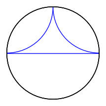
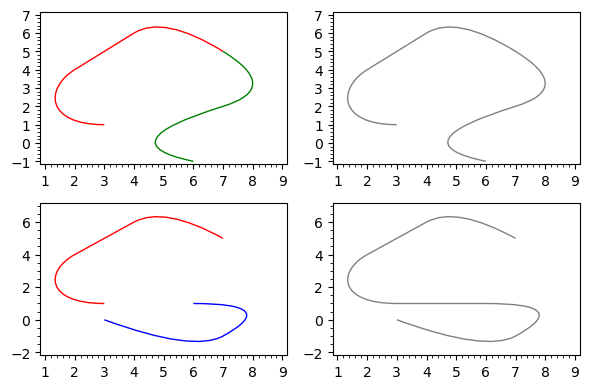
Notice that the boundary disc looks like it was plotted three times. It is indeed the case, as we shall see. A hint, in the Sage REPL (in the terminal) is that it mentions "6 graphics primitives", which we can guess are the three geodesics and three copies of the boundary circle.

To get started, let's give names to the geodesics.

sage: a, b, c = lines

Explore their methods using the TAB key: a.<TAB> reveals the method plot.

Give a name to the plots:

sage: pa, pb, pc = a.plot(), b.plot(), c.plot()

Explore their methods using the TAB key: pa.<TAB> reveals the method description.

sage: print(pa.description())
Arc with center (1.0,1.0) radii (1.0,1.0) angle 0.0
inside the sector (3.141592653589793,4.71238898038469)
Circle defined by (0.0,0.0) with r=1.0
sage: print(pb.description())
Arc with center (-1.0,1.0) radii (1.0,1.0) angle 0.0
inside the sector (-1.5707963267948966,0.0)
Circle defined by (0.0,0.0) with r=1.0
sage: print(pc.description())
Line defined by 2 points:   [(-1.0, 0.0), (1.0, 0.0)]
Circle defined by (0.0,0.0) with r=1.0

We see each description consists of two lines, one for an arc and a second one for the boundary circle. So indeed it was being plotted three times.

Could we get rid of the boundary circle? Exploring the plot method using a.plot? reveals the optional keyword boundary which defaults to True. Using False instead, we can get rid of the extra circles.

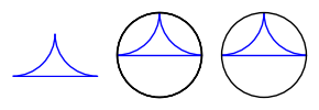
sage: pa_nb = a.plot(boundary=False)
sage: pb_nb = b.plot(boundary=False)
sage: pc_nb = c.plot(boundary=False)
sage: abc0 = pa_nb + pb_nb + pc_nb  # no boundary
sage: abc3 = pa + pb + pc  # boundary plotted 3 times
sage: abc1 = pa_nb + pb_nb + pc  # boundary plotted once
sage: abc_013 = graphics_array([abc0, abc3, abc1])
sage: abc_013.show(figsize=3)

Can we get the boundary by itself? By exploring DD with DD.<TAB>, we find a method get_background_graphic which gives it.

Besides the multiple plotting of the boundary, we observe that:

• geodesics through the origin are euclidean line segments; their description gives their two endpoints
• geodesics not through the origin are euclidean circle arcs; their description gives center and radius

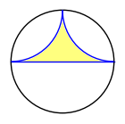
This gives the idea of using region_plot (see the Sage graphics tour).

For that, we write inequalities to describe the region

• inside the unit circle:
• outside the circles for sides not through the origin:
• on the appropriate side of the lines for sides through the origin:

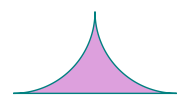
In our case:

sage: boundary = DD.get_background_graphic()
sage: p = sum(line.plot(boundary=False) for line in lines)
sage: x, y = SR.var('x, y')
sage: ieqs = [x^2 + y^2 < 1,
....:         (x - 1)^2 + (y - 1)^2 > 1,
....:         (x + 1)^2 + (y - 1)^2 > 1,
....:         y > 0]
sage: opt = {'incol': '#ffff7f', 'axes': False}
sage: inside = region_plot(ieqs, (x, -1, 1), (y, 0, 1), **opt)
sage: g = boundary + inside + p
sage: g.save('disc_triangle_filled_in.png', figsize=2)
sage: g.show(figsize=2)

Polygon plotting function using Sage's region plot function

Based on our exploration, we write the following function:

def discgon(points, color='teal', fill_color='plum',
            plot_points=65, thickness=1.5, **opt):
    r"""
    Return a hyperbolic polygon in the disc model as a graphics object.

    INPUT:

    - ``points`` -- a list of complex numbers in the unit disc,
      consecutive vertices of a convex hyperbolic polygon
    - ``color`` -- (default: 'teal') line thickness for sides
    - ``fill_color`` -- (default: 'plum') fill color for polygon
    - ``plot_points`` -- (default: 257) number of points on the arcs
    - ``thickness`` -- (default: 1.5) line thickness for sides
    - ``opt`` -- optional extra plotting options

    EXAMPLES::

        sage: a = [1, I, -1]
        sage: b = [0, 1/2, 1/2 + 1/2*I, 1/2*I]
        sage: c = [0, 1/2, 1/2 + 1/2*I, I, -1/2 + 1/2*I]
        sage: d = [(3/4 if k % 2 else 1)*E(8)^k for k in range(8)]
        sage: abcd = graphics_array([discgon(p) for p in [a, b, c, d]])
        sage: abcd.show(figsize=5)
        Launched png viewer for Graphics Array of size 1 x 4
        sage: fivegons = [discgon([r/4*E(5)^k for k in range(5)])
        ....:             for r in range(1, 5)]
        sage: fives = graphics_array(fivegons)
        sage: fives.show(figsize=5)
        Launched png viewer for Graphics Array of size 1 x 4
    """
    line_opt = {'color': color, 'thickness': thickness}
    fill_opt = {'incol': fill_color, 'plot_points': plot_points}
    n = len(points)
    if n < 3:
        raise ValueError(f"need >= 3 points for polygon, got {n}")
    xy = [(real(z), imag(z)) for z in points]
    xx, yy = zip(*(list(z) for z in xy))
    xab = min(xx), max(xx)
    yab = min(yy), max(yy)
    x, y = SR.var('x, y')
    DD = HyperbolicPlane().PD()
    relations = [x^2 + y^2 < RDF.one()]
    side_plots = []
    for k, q in enumerate(points, start=-1):
        p = points[k]
        pq = DD.get_geodesic(p, q).plot(boundary=False, **line_opt, **opt)
        side_plots.append(pq)
        d = pq.description()
        if d.startswith('Arc'):
            xc, yc, r, _ = (RDF(z) for s in d.split(')')[:-2]
                            for z in s.split('(')[1].split(','))
            relations.append((x - xc)^2 + (y - yc)^2 > r^2)
        elif d.startswith('Line'):
            xa, ya, xb, yb = (RDF(z) for s in d.split(')')[:-1]
                              for z in s.split('(')[1].split(','))
            a = yb - ya
            b = xa - xb
            lin_form = a * x + b * y
            aff_fc = lin_form - lin_form.subs({x: p.real(), y: p.imag()})
            a, r, j = max((abs(ft), ft, j)
                          for j, t in enumerate(xy)
                          for ft in [aff_fc.subs({x: t[0], y: t[1]})])
            relations.append(sign(r)*aff_fc > 0)
        else:
            raise ValueError("unexpected side type")
    inside = region_plot(relations, xab, yab, **fill_opt, **opt)
    return sum(side_plots, DD.get_background_graphic(**opt) + inside)

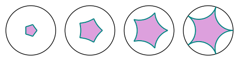
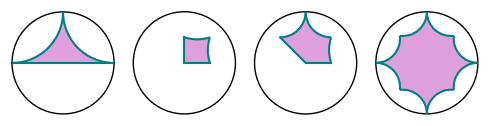
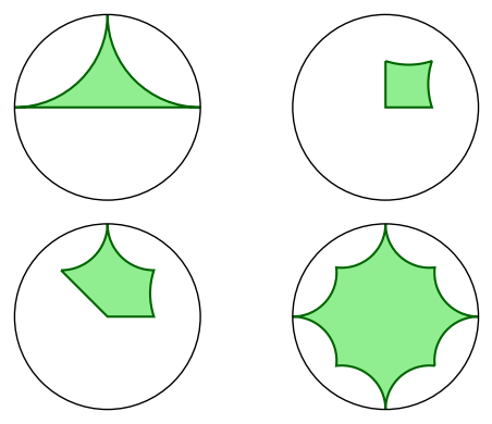
We test our function:

sage: a = [1, I, -1]
sage: b = [0, 1/2, 1/2 + 1/2*I, 1/2*I]
sage: c = [0, 1/2, 1/2 + 1/2*I, I, -1/2 + 1/2*I]
sage: d = [(3/4 if k % 2 else 1)*E(8)^k for k in range(8)]
sage: abcd = graphics_array([discgon(p) for p in [a, b, c, d]])
sage: abcd.show(figsize=5)
Launched png viewer for Graphics Array of size 1 x 4

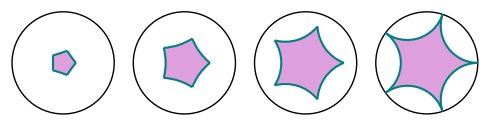
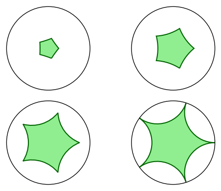
sage: fives = [[r/4*E(5)^k for k in range(5)] for r in range(1, 5)]
sage: fivegons = graphics_array([discgon(f) for f in fives])
sage: fivegons.show(figsize=5)
Launched png viewer for Graphics Array of size 1 x 4

Improvement ideas

The approach above is somewhat unsatisfactory for several reasons.

First, the region plot poorly fills near acute vertices, especially if we sample too few points.

Second, sampling is wasteful in itself, since we already know the outline of the region to plot.

This suggests approximating that outline by a euclidean polygon and using Sage's 2D polygon plotting function, which can fill.

Replacing sides by polygonal lines is easy: sides through the origin are already segments, and those not through the origin are circle arcs which we can approximate by polygonal lines.

Polygon plotting function using Sage's (euclidean) 2D polygon function

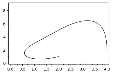
Let us warm up with the initial example. The side descriptions not only include the center and radius of the corresponding euclidean circle, but also the two extreme angles for the arc.

So we can write something like:

sage: nsteps = 64
sage: s, t = (3.141592653589793, 4.71238898038469)
sage: step = (t - s) / nsteps
sage: stop = s - step / 2
sage: aa = [(1 + cos(x), 1 + sin(x)) for x in srange(t, stop, -step)]
sage: s, t = (-1.5707963267948966, 0.0)
sage: step = (t - s) / nsteps
sage: stop = s - step / 2
sage: bb = [(-1 + cos(x), 1 + sin(x)) for x in srange(t, stop, -step)]
sage: cc = [(-1.0, 0.0), (1.0, 0.0)]
sage: abc = aa + bb + cc
sage: abc_gon = polygon2d(abc, color='plum', edgecolor='teal', axes=False)
sage: abc_gon.show(figsize=2)

Turning this into a function, we get:

def disc_ngon(points, color='teal', fill_color='plum',
              thickness=1.5, nsteps=256, **opt):
    r"""
    Return a hyperbolic polygon in the disc model as a graphics object.

    INPUT:

    - ``points`` -- list of complex numbers in the unit disc for vertices
      of a convex hyperbolic polygon listed counterclockwise
    - ``color`` -- (default: 'teal') the line color for the sides
    - ``fill_color`` -- (default: 'plum') the fill color for the polygon
    - ``thickness`` -- (default: 1.5) the line thickness for the sides
    - ``nsteps`` -- (default: 256) number of steps for circular sides
    - ``opt`` -- optional extra options

    Circular sides are turned into polygonal lines with ``nsteps`` segments
    for filling the polygon.

    EXAMPLES::

        sage: a = [1, I, -1]
        sage: b = [0, 1/2, 1/2 + 1/2*I, 1/2*I]
        sage: c = [0, 1/2, 1/2 + 1/2*I, I, -1/2 + 1/2*I]
        sage: d = [(3/4 if k % 2 else 1)*E(8)^k for k in range(8)]
        sage: abcd = graphics_array([discgon(p) for p in [a, b, c, d]])
        sage: abcd.show(figsize=5)
        Launched png viewer for Graphics Array of size 1 x 4
        sage: fivegons = [discgon([r/4*E(5)^k for k in range(5)])
        ....:             for r in range(1, 5)]
        sage: fives = graphics_array(fivegons)
        sage: fives.show(figsize=5)
        Launched png viewer for Graphics Array of size 1 x 4
    """
    line_opt = {'color': color, 'thickness': thickness}
    fill_opt = {'color': fill_color, 'thickness': 0}
    n = len(points)
    if n < 3:
        raise ValueError(f"need >= 3 points for polygon, got {n}")
    xy = [(real(z), imag(z)) for z in points]
    DD = HyperbolicPlane().PD()
    side_plots = []
    vertices = []
    for k, q in enumerate(points, start=-1):
        p = points[k]
        vertices.append(xy[k])
        pq = DD.get_geodesic(p, q).plot(boundary=False, **line_opt, **opt)
        side_plots.append(pq)
        d = pq.description()
        if d.startswith('Arc'):
            xc, yc, r, _, s, t = (RDF(z) for s in d.split(')')[:-1]
                                  for z in s.split('(')[1].split(','))
            step = (t - s) / nsteps
            vertices.extend([(xc + r*cos(x), yc + r*sin(x))
                             for x in srange(t + step/2, s, -step)])
    inside = polygon2d(vertices, **fill_opt, **opt)
    return sum(side_plots, DD.get_background_graphic(**opt) + inside)

We test our function:

sage: a = [1, I, -1]
sage: b = [0, 1/2, 1/2 + 1/2*I, 1/2*I]
sage: c = [0, 1/2, 1/2 + 1/2*I, I, -1/2 + 1/2*I]
sage: d = [(3/4 if k % 2 else 1)*E(8)^k for k in range(8)]
sage: abcd = graphics_array([disc_ngon(p) for p in [a, b, c, d]])
sage: abcd.show(figsize=5)
Launched png viewer for Graphics Array of size 1 x 4

sage: fives = [[r/4*E(5)^k for k in range(5)] for r in range(1, 5)]
sage: fivegons = graphics_array([disc_ngon(f) for f in fives])
sage: fivegons.show(figsize=5)
Launched png viewer for Graphics Array of size 1 x 4