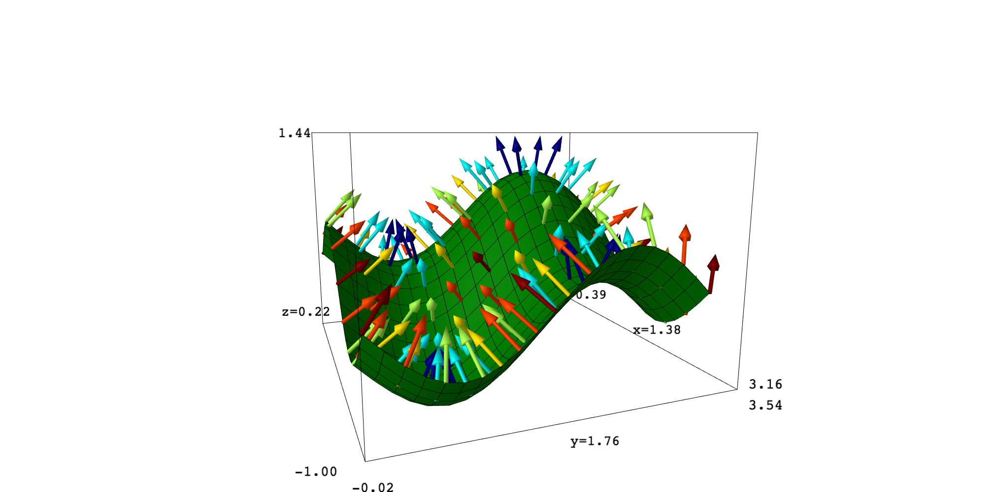
I think that SageMath does not have a function behaving as you want, but you can define your own. In fact, it seems that this is what you are doing. On my side, I have ended with the following code which perhaps may be useful. It can be seem, as well as the examples, in this SageMath Cell. The image at the end corresponds to the second example.
def gradient_plot(fun, range_x, range_y, plot_points=10, color="red", radius=1/50, scale=1):
    r"""
    Plot gradient vectors of a bivariate function on points of its graph.
    Arguments:
    - fun: a symbolic expression corresponding to the function
    - range_x and range_y: tuples of the form (var, min_value, max_value); the variables of
      fun should be the first elements of these tuples
    Options:
    - plot_points: number of points in each direction; it can be a number or a list or a
      tuple
    - color: a specific color for all vectors or "gradient"; in this case, vectors are
      colored depending on their norms
    - radius: radius of the arrow
    - scale: a factor to increase or decrease the length of the arrows

    Example:
    f(u,v) = u^2-v^2
    g = gradient_plot(f(u,v), (u,-1,1), (v,-1,1), scale=0.5)
    s = plot3d(f(u,v), (u,-1,1), (v,-1,1), mesh=True)
    show(g+s)

    Another example:
    var("x,y")
    fun = cos(x+y)*sin(x-y)
    x1, x2, y1, y2 = 0, pi, 0, pi
    surface = plot3d(fun, (x,x1,x2), (y,y1,y2), mesh=True, color="green", plot_points=21)
    gradients = gradient_plot(fun, (x,x1,x2), (y,y1,y2), plot_points=11,
                                scale=0.5, color="gradient", radius=0.02)
    show(surface+gradients)
    """

    # Process arguments
    # -----------------
    # fun
    fx, fy = fun.gradient()

    # ranges
    var_x, xmin, xmax = range_x
    var_y, ymin, ymax = range_y

    # plot_points
    if isinstance(plot_points, (list, tuple)):
        nx, ny = plot_points
    else:
        nx = ny = plot_points

    # color
    if color=="gradient":
        color = "red"
        gradient_colors = True
    else:
        gradient_colors = False

    # Compute gradient vectors at surface points and obtain the
    # corresponding arrows to be plotted
    # Gradient norms are also stored
    norms = []
    arrows = []
    dx, dy = (xmax-xmin)/(nx-1), (ymax-ymin)/(ny-1)
    iter_x = [xmin,xmin+dx,..,xmax]
    iter_y = [ymin,ymin+dy,..,ymax]
    for xx in iter_x:
        for yy in iter_y:
            dic = {var_x: xx, var_y: yy}
            p = [xx, yy, fun(dic)]
            v = vector([-fx(dic), -fy(dic), 1])
            nv = norm(v).n()
            norms.append(nv)
            v = scale*v/nv
            arrows.append(arrow((0,0,0),v, color=color, radius=radius).translate(p))

    # If required, modify arrow colors depending on the gradient norm.
    # Colors range from dark blue (small norm) to dark red (big norm)
    if gradient_colors:
        nvmin, nvmax = min(norms), max(norms)
        if nvmin==nvmax: nvmin = 0
        for i in range(len(arrows)):
            icol = (norms[i]-nvmin)/(nvmax-nvmin)
            vcol = colormaps.jet(icol)[:-1]
            arrows[i].set_texture(color=vcol)
    # End
    return sum(arrows)
Edit. The line fx, fy = fun.gradient() fails if fun is a constant or only contains one variable. So it is better to replace
fx, fy = fun.gradient()
var_x, xmin, xmax = range_x
var_y, ymin, ymax = range_y
by
var_x, xmin, xmax = range_x
var_y, ymin, ymax = range_y
fx, fy = fun.diff(var_x), fun.diff(var_y)

