Ask Your Question
2

Arrow length goes wild near poles in vector field plot

asked 2019-04-13 11:11:53 +0200

stockh0lm gravatar image

updated 2019-04-13 23:56:55 +0200

slelievre gravatar image

Running this piece of code

x, y = var('x y')
f = 1/sqrt(x^2 + y^2)
grad = f.gradient([x, y])
plot_vector_field(grad, (x, -1, 1), (y, -1, 1)).show()
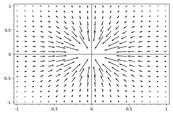
gives me this

image description

As you can see the arrows very close to the pole "cross out" the whole pic. Obviously they are very large vectors, but they do harm the overall image. I have other plots where its worse. How can I work around that? Can I blank out the direct proximity of the pole, somehow? Can I limit the vectors' length? How?

edit retag flag offensive close merge delete

2 Answers

Sort by ยป oldest newest most voted
2

answered 2019-04-13 11:35:43 +0200

rburing gravatar image

updated 2019-04-13 19:01:29 +0200

Yes, you can limit the proximity to the pole:

my_grad = [lambda x,y: grad[0].subs(x=x,y=y) if x^2 + y^2 > 0.1 else None,
           lambda x,y: grad[1].subs(x=x,y=y) if x^2 + y^2 > 0.1 else None]
plot_vector_field(my_grad, (x,-1,1), (y,-1,1)).show()

limit proximity to pole

or limit the length of the vectors:

my_grad = [lambda x,y: grad[0].subs(x=x,y=y) if abs(grad.subs(x=x,y=y)) < 7 else None,
           lambda x,y: grad[1].subs(x=x,y=y) if abs(grad.subs(x=x,y=y)) < 7 else None]
plot_vector_field(my_grad, (x,-1,1), (y,-1,1)).show()

limit vector length

edit flag offensive delete link more

Comments

neat! thank you, rburing! I do need to figure out those lambda functions...

Could you please explain a little what happens in those lambda functions? especially the .subs() is confusing to me. Also the "else None" seems to be the limitation and only happens if abs(x) + abs(y) exceed the limit, but how does it limit, really? it does not replace anything in that case, does it? Is my_grad just a copy of grad? and it only copies if it does not exceed? does the subs() only happen in case if() is true?

is it perhaps like this (in pseudo code): if (grad_len < 7) then (copy x and y), else (don't). why would you have two subs in the second case, not just one as in the first?

stockh0lm gravatar imagestockh0lm ( 2019-04-13 12:50:00 +0200 )edit

Your grad is a pair of symbolic expressions; my_grad is a pair of functions of x and y (defined inline, using lambda). The function plot_vector_field accepts both forms; in the first case it substitutes numeric values into the expressions and in the second case it calls the functions with numeric arguments. The functions in my_grad return the same result as grad would (by substituting into the expressions), but when some condition is not satisfied they return None instead (which causes plot_vector_field not to plot the vector).

In the second example subs() is used in the condition, because it depends not just on the position (the numeric x and y) but also the vector length (i.e. on grad or grad_len, into which the numeric x and y are substituted).

rburing gravatar imagerburing ( 2019-04-13 14:04:09 +0200 )edit

thanks so kindly!

stockh0lm gravatar imagestockh0lm ( 2019-04-13 16:42:16 +0200 )edit

wow, i tried the second approach (so much more flexible!) and it almost brought my box to the knees - out of memory and CPU to the max... the simple example worked for me, too, but my real gradient field didn't.

what is so insanely memory intensive about this?

stockh0lm gravatar imagestockh0lm ( 2019-04-13 18:20:06 +0200 )edit

It was using the symbolic expression for the length of the gradient vector, which was not a very good idea. I updated the answer. Now the gradient vector is computed numerically first, and then the length is taken. Another optimization is to use the conditional (if ... else None) only on the first coordinate. There is still some inefficiency since one component of the numerical gradient is computed twice (once for the condition, and once for the return value). Let me know if it is still too inefficient.

rburing gravatar imagerburing ( 2019-04-13 19:11:28 +0200 )edit
3

answered 2019-04-13 18:47:08 +0200

eric_g gravatar image

An alternative is to define f on the Euclidean plane minus a small disk around the origin:

E.<x,y> = EuclideanSpace()
U = E.open_subset('U', coord_def={E.cartesian_coordinates(): x^2+y^2>0.2})
f = U.scalar_field(1/sqrt(x^2+y^2))
grad = f.gradient()
grad.plot(max_range=1, scale=0.1)

gradient plot

edit flag offensive delete link more

Your Answer

Please start posting anonymously - your entry will be published after you log in or create a new account.

Add Answer

Question Tools

2 followers

Stats

Asked: 2019-04-13 11:11:53 +0200

Seen: 572 times

Last updated: Apr 13 '19