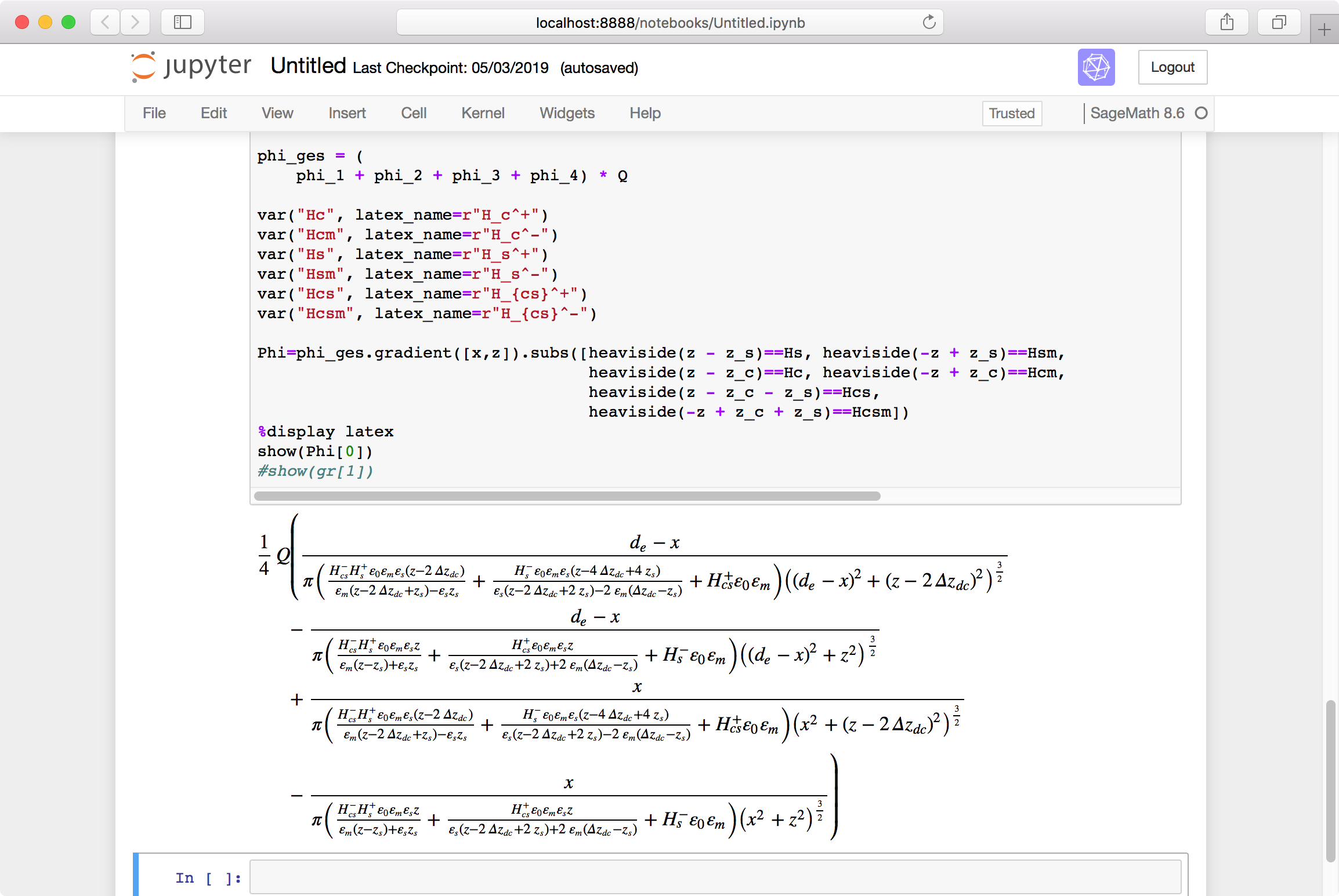
grad() at glacial speed

asked 2019-03-31 16:00:08 +0200

stockh0lm
270 ●4 ●8 ●26

updated 2019-03-31 20:11:10 +0200

I try to calculate grad() in this worksheet. It is really slow, and so far has not completed. Are there ways to speed it up? It should be mostly calculating the derivatives in x and z directions. Shouldnt that be comparatively quick?

x,z, z_c, z_s, d_e, epsilon_m, epsilon_s, v_ges, Q, U, a =var('x z z_c z_s d_e epsilon_m epsilon_s v_ges Q U a')
z_c = var('z_c', latex_name=r'\varDelta z_{dc}')
z_m = var('z_m', latex_name=r'\varDelta z_{ds}')

epsilon_0 = var('epsilon_0', latex_name=r'\varepsilon_0')
epsilon_s = var('epsilon_s', latex_name=r'\varepsilon_s')
epsilon_m = var('epsilon_m', latex_name=r'\varepsilon_m')

epsilon_Ersatz(epsilon_1,epsilon_2,d_1,d_2) = epsilon_1*epsilon_2*(d_1+d_2)/(d_1*epsilon_2+d_2*epsilon_1)

phi(epsilon, Q, r) = 1/(4*pi*epsilon)*Q/r
latex( SR.symbol ('phi') == phi)

phi_1 = phi(heaviside( z_s -z )                           * epsilon_0*epsilon_m
          + heaviside( z- z_s ) * heaviside(z_c + z_s -z) * epsilon_0*epsilon_Ersatz(epsilon_m, epsilon_s, z_s            , z-z_s)
          + heaviside( z -(z_c + z_s))                    * epsilon_0*epsilon_Ersatz(epsilon_m, epsilon_s, (z-2*(z_c-z_s)), 2*(z_c-z_s)),
          1, sqrt(x^2 + z^2)
)
phi_2 = phi(heaviside( z_s -z )                           * epsilon_0*epsilon_m
          + heaviside( z- z_s ) * heaviside(z_c + z_s -z) * epsilon_0*epsilon_Ersatz(epsilon_m, epsilon_s, z_s            , z-z_s)
          + heaviside( z -(z_c + z_s))                    * epsilon_0*epsilon_Ersatz(epsilon_m, epsilon_s, ( z -2*(z_c-z_s)), 2*(z_c-z_s)),
          -1, sqrt((d_e-x)^2 + z^2)
)
phi_3 = phi(heaviside( z_s -z)                            * epsilon_0*epsilon_Ersatz(epsilon_m, epsilon_s, (-z +2*(z_c-z_s)), 2*(z_c-z_s))
          + heaviside( z- z_s ) * heaviside(z_c + z_s -z) * epsilon_0*epsilon_Ersatz(epsilon_m, epsilon_s, z_s              , 2*z_c-z_s -z)
          + heaviside( z -(z_c + z_s))                    * epsilon_0*epsilon_m,
          -1, sqrt((2*z_c-z)^2+x^2))
phi_4 = phi(heaviside( z_s -z)                            * epsilon_0*epsilon_Ersatz(epsilon_m, epsilon_s, (-z +2*(z_c-z_s)), 2*(z_c-z_s))
          + heaviside( z- z_s ) * heaviside(z_c + z_s -z) * epsilon_0*epsilon_Ersatz(epsilon_m, epsilon_s, z_s              , 2*z_c-z_s -z)
          + heaviside( z -(z_c + z_s))                    * epsilon_0*epsilon_m,    
          1, sqrt((2*z_c-z)^2+(d_e -x)^2))

phi_ges = (
    phi_1 + phi_2 + phi_3 + phi_4) * Q
latex(phi_ges)
from sage.manifolds.operators import *   # to get the operators grad, div, curl, etc.
S.<x,z> = EuclideanSpace(2)
Phi = S.scalar_field(phi_ges, name='Phi')
print((-grad(Phi)).display())

edit retag flag offensive close merge delete

add a comment

3 Answers

Sort by » oldest newest most voted

answered 2019-04-01 17:08:39 +0200

eric_g
8209 ●10 ●61 ●162 https://luth.obspm.fr/...

updated 2019-04-03 23:34:38 +0200

Using SageMath 8.7, I confirm that the command grad(Phi) runs for ever... Actually, this is not the computation of the gradient by itself that takes time but its simplification. The quantity phi_ges from which the scalar field Phi is formed is a quite lengthy symbolic expression. Sage evaluates

diff(phi_ges, z)

quite fast but then the command

diff(phi_ges, z).simplify_full()

runs for ages... It turns out that grad(Phi) is using a simplification sequence pretty similar to simplify_full() (the details are here) to simplify its output. Hence the observed behavior. Maybe this is an issue of the simplification of long symbolic expressions involving Heaviside functions in Sage...

EDIT: a possible workaround is to replace simplify_chain_real by the mere simplify function as the simplifying function associated to the default chart (x,z) of the Euclidean space S; to do this, it suffices to insert the line

S.default_chart()._calc_method._simplify_dict['SR'] = simplify

just after the definition S.<x,z> = EuclideanSpace(2).

Explanations:

S.default_chart() is the chart of Cartesian coordinates $(x,z)$ on the Euclidean plane $S$
_calc_method is the calculus method, i.e. the tool managing the symbolic backend that is used when perfoming calculations with the chart $(x,z)$: either the symbolic ring SR (SageMath's default) or SymPy
_simplify_dict is the dictionary of simplifying functions associated to each symbolic backend: by default, _simplify_dict['SR'] = simplify_chain_real and _simplify_dict['sympy'] = simplify_chain_real_sympy
the function simplify in the right-hand side of the suggested command is SageMath's minimal simplifying function: it is fast, but it does not do much. You can replace it by any function that maps a symbolic expression to another symbolic expression.

With the above command,

%time print((-grad(Phi)).display())

returns

CPU times: user 498 ms, sys: 18.6 ms, total: 517 ms
Wall time: 396 ms

EDIT (3 April 2019): motivated by your question, I've opened the Trac ticket #27601 to allow for an easy modification of the simplifying function.

edit flag offensive delete link

Comments

can you suggest a more speedy simplification algorithm, perhaps in sympy?

stockh0lm ( 2019-04-01 17:53:52 +0200 )edit

I've edited my answer, indicating how to replace simplify_chain_real by the much more speedy simplify (but less efficient in simplifying).

eric_g ( 2019-04-01 23:55:23 +0200 )edit

thank you for opening a ticket for this.

stockh0lm ( 2019-04-04 12:12:25 +0200 )edit

add a comment

answered 2019-04-02 00:47:11 +0200

Juanjo

3203 ●5 ●41 ●85

Perhaps you could stick to the symbolic ring and compute the gradient just with phi_ges.gradient([x,z]). It is quite fast. Then you can grasp how the gradient is by displaying both components of the gradient vector. The second component is a bit "terrific", but the first one is quite human readable as shown in the following screen capture:

image description

Please note that $H^+_s$, $H^-_s$ and so on represent Heaviside functions evaluated at different arguments (see the var functions and the subs method in the picture). I wonder if this expression can be really simplified.

edit flag offensive delete link

Comments

i don't think the expression can be simplified beyond simple things like pulling out 1/pi.

stockh0lm ( 2019-04-02 11:01:51 +0200 )edit

That Hs+, Hs- etc notation is great. i didnt know you could do substitutions like that. Is it also possible to color that specific term in the (latex) output, so that the different cases are easily recognized?

stockh0lm ( 2019-04-02 13:05:20 +0200 )edit

Yes, of course. For example, you could replace

var("Hcsm", latex_name=r"H_{cs}^-")

var("Hcsm", latex_name=r"\color{red}{H_{cs}^-}")

to get $\color{red}{H_{cs}^-}$.

Juanjo ( 2019-04-02 14:50:21 +0200 )edit

thank you!

I realize that my question was not as clear as it could have been. I would like to color the whole term in which Hs+ (etc) is a factor, not just Hs+ itself. That way i could visualize which terms belong together to the same case (corresponding to the same geometric area). So the color would need to taint the whole product that Hs+ is a factor of. Is that possible, too?

stockh0lm ( 2019-04-03 14:42:32 +0200 )edit

add a comment

answered 2019-03-31 19:36:47 +0200

Emmanuel Charpentier
7057 ●6 ●46 ●137

updated 2019-03-31 22:49:44 +0200

Stockholm,

Could you try to create a minimal exemple exhibiting the behaviour you complain of ?

And again:

e = var('e', latex_name=r'\varepsilon')

At the (assumed) risk of monkeying the (British) Commons : No, no, no, no, no, no, no, no.

And no.

HTH,

EDIT : WorksForMe(TM) in sage 8.8.beta0 (with a very suspicious result : I'm afraid that you don't use manifolde as they are intended to be...):

sage: %time print((-grad(Phi)).display())
-grad(Phi) = 0
CPU times: user 994 µs, sys: 20 µs, total: 1.01 ms
Wall time: 1.02 ms

sage: Phi.display()
Phi: E^2 --> R
   (x, z) |--> 1/4*Q*(1/(pi*(epsilon_0*epsilon_m*epsilon_s*(z - 2*z_c)*heaviside(z - z_s)*heaviside(-z + z_c + z_s)/(epsilon_m*(z - 2*z_c + z_s) - epsilon_s*z_s) + epsilon_0*epsilon_m*epsilon_s*(z - 4*z_c + 4*z_s)*heaviside(-z + z_s)/(epsilon_s*(z - 2*z_c + 2*z_s) - 2*epsilon_m*(z_c - z_s)) + epsilon_0*epsilon_m*heaviside(z - z_c - z_s))*sqrt((d_e - x)^2 + (z - 2*z_c)^2)) - 1/(pi*(epsilon_0*epsilon_m*epsilon_s*z*heaviside(z - z_s)*heaviside(-z + z_c + z_s)/(epsilon_m*(z - z_s) + epsilon_s*z_s) + epsilon_0*epsilon_m*epsilon_s*z*heaviside(z - z_c - z_s)/(epsilon_s*(z - 2*z_c + 2*z_s) + 2*epsilon_m*(z_c - z_s)) + epsilon_0*epsilon_m*heaviside(-z + z_s))*sqrt((d_e - x)^2 + z^2)) - 1/(pi*(epsilon_0*epsilon_m*epsilon_s*(z - 2*z_c)*heaviside(z - z_s)*heaviside(-z + z_c + z_s)/(epsilon_m*(z - 2*z_c + z_s) - epsilon_s*z_s) + epsilon_0*epsilon_m*epsilon_s*(z - 4*z_c + 4*z_s)*heaviside(-z + z_s)/(epsilon_s*(z - 2*z_c + 2*z_s) - 2*epsilon_m*(z_c - z_s)) + epsilon_0*epsilon_m*heaviside(z - z_c - z_s))*sqrt(x^2 + (z - 2*z_c)^2)) + 1/(pi*(epsilon_0*epsilon_m*epsilon_s*z*heaviside(z - z_s)*heaviside(-z + z_c + z_s)/(epsilon_m*(z - z_s) + epsilon_s*z_s) + epsilon_0*epsilon_m*epsilon_s*z*heaviside(z - z_c - z_s)/(epsilon_s*(z - 2*z_c + 2*z_s) + 2*epsilon_m*(z_c - z_s)) + epsilon_0*epsilon_m*heaviside(-z + z_s))*sqrt(x^2 + z^2)))

What is E ?

edit flag offensive delete link

Comments

lol, the e is not even used. It escaped when I replaced the used instances of epsilon. fixed now.

An important part of my question is how to speed up this calculation. Simple grad()s are rather quick, but still way slower then doing derivatives.

Also my local experiments seem to indicate that it takes way longer to do grad(phi_1+phi_2+phi_3+phi_4) then grad(phi_1)+grad(phi_2)+grad(phi_3)+grad(phi_4). For that reason it seems relevant to look as a pseudo-complex example like this.

stockh0lm ( 2019-03-31 20:29:39 +0200 )edit

-grad(Phi)= 0 ?!? That would mean that I screwed up the equation, because this is a field that certainly has a result (!= 0).

And did you need to do anything that it returned that result that quickly? that answer came lightning fast!

What makes you say I use the manifold incorrectly? What do I do wrong?

I run sage 8.6.

stockh0lm ( 2019-03-31 23:35:17 +0200 )edit

E is the euclidian space that i define earlier.

stockh0lm ( 2019-04-01 10:23:56 +0200 )edit

add a comment

Your Answer

Please start posting anonymously - your entry will be published after you log in or create a new account.

Add Answer

grad() at glacial speed

3 Answers

Comments

Comments

Comments

Your Answer

Question Tools

Stats

grad() at glacial speed edit

3 Answers

Comments

Comments

Comments

Your Answer

Question Tools

Stats

grad() at glacial speed