Revision history [back]

In your expression, the x^3 terme dominates the other ones for large (absolute values of) x. This can be seen by computing their ratios for the limits you used :

sage: [(x^3/(-2*x^2+5*x+6)).subs(x=u).n(digits=3) for u in (-200, 200)]
[98.8, -101.]

In other words, the difference between the plot of your expression ant the plot of x^3 is way too small (1/200th of the ordinate scale) to be perceptible...

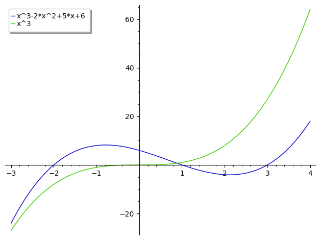
As pointed out by @tolga, restricting your plot to a small region around the roots makes this more visible :

sage: plot([x^3-2*x^2-5*x+6, x^3], (x, -3, 4), legend_label=["x^3-2*x^2+5*x+6", "x^3"])

HTH,

In your expression, the x^3 terme dominates the other ones for large (absolute values of) x. This can be seen by computing their ratios for the limits you used :

sage: [(x^3/(-2*x^2+5*x+6)).subs(x=u).n(digits=3) for u in (-200, 200)]
[98.8, -101.]

In other words, the difference between the plot of your expression ant the plot of x^3 is way too small (1/200th of the ordinate scale) to be perceptible...

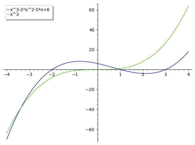
As pointed out by @tolga, restricting your plot to a small region around the roots makes this more visible :

sage: plot([x^3-2*x^2-5*x+6, x^3], (x, -3, 4), legend_label=["x^3-2*x^2+5*x+6", "x^3"])

HTH,