Revision history [back]
| | 1 | initial version |
As observed in the question,
the solution contains a parameter _C.
That parameter does not get declared globally, so we need to do that before we can use it.
Here is one way using subs.
Define the variable, the function, the differential equation.
sage: x = SR.var('x')
sage: y = function('y')
sage: yprime = diff(y(x), x)
sage: de = (x^2)*yprime == y(x)
sage: de
x^2*diff(y(x), x) == y(x)
Solve.
sage: g(x) = desolve(de, [y(x), x])
sage: g
x |--> _C*e^(-1/x)
Declare the parameter as a symbolic variable.
sage: _C = SR.var('_C')
Plot solutions for a range of values of the parameter.
sage: dessin = plot([g(x).subs({_C: c}) for c in srange(-8, 8, 0.4)], (x, -3, 3))
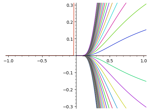
| | 2 | No.2 Revision |
As observed in the question,
the solution contains a parameter _C.
That parameter does not get declared globally, so we need to do that before we can use it.
Here is one way using subs.
Define the variable, the function, the differential equation.
sage: x = SR.var('x')
sage: y = function('y')
sage: yprime = diff(y(x), x)
sage: de = (x^2)*yprime == y(x)
sage: de
x^2*diff(y(x), x) == y(x)
Solve.
sage: g(x) = desolve(de, [y(x), x])
sage: g
x |--> _C*e^(-1/x)
Declare the parameter as a symbolic variable.
sage: _C = SR.var('_C')
Plot solutions for a range of values of the parameter.
sage: dessin = plot([g(x).subs({_C: c}) for c in srange(-8, 8, 0.4)], (x, -3, 3))
sage: dessin.show(xmin=-1, xmax=1, ymin=-0.3, ymax=0.3)
Launched png viewer for Graphics object consisting of 80 graphics primitives
