Revision history [back]

Assume that we have $n+1$ data points $(x_0,y_0),\ldots,(x_n,y_n)$, with $x_i\ne x_j$ for $i\ne j$. Then, there exists a unique polynomial $f$ of degree $\leq n$ such that $f(x_i)=y_i$ for $i=0,\ldots,n$. This is the Lagrange polynomial that interpolates the given data. In his answer, @dsejas has shown a method to compute it. In the current case, since $n=3$, the interpolating polynomial has degree $\leq3$; in fact, it is $f(x)=x^2$.

If $f(x)=a_0+a_1x+\cdots+a_nx^n$, it follows from the interpolation conditions that the coefficients are the solution of the linear system $A\mathbf{x}=\mathbf{b}$, where $A=(x_i^j)$ (the element of $A$ at row $i$ and column $j$ is $x_i^j$) and $\mathbf{b}=(y_i)$. This is not the best way to get $a_0,\ldots,a_n$, since $A$ is usually an ill conditioned matrix. However, it is interesting to point out that from a theoretical viewpoint.

If one has $m$ data points and still wants to fit them using a polynomial of degree $n$, with $n\leq m$, the linear system $A\mathbf{x}=\mathbf{b}$ is overdetermined (there are more equations than unknowns). In such a case, one can perform a least squares fitting, trying to minimize the interpolation errors, that is, one seeks for the minimum of $$E(a_0,a_1,\ldots,a_n)=\sum_{i=0}^m (f(x_i)-y_i)^2.$$ The minimum is given by the solution of the linear system $$ \nabla E(a_0,a_1,\ldots,a_n)=\mathbf{0},$$ which is simply $A^TA\mathbf{x}=A^T\mathbf{b}$. This is what @Cyrille, in fact, proposes in his answer... computing explicitly $E(a_0,a_1,\ldots,a_n)$ as well as its partial derivatives, which is completely unnecessary. In fact, if the system $A\mathbf{x}=\mathbf{b}$ has a unique solution, which is the case under discussion, the system $A^TA\mathbf{x}=A^T\mathbf{b}$ yields exactly the same solution. So, the function in @Cyrille's answer is just the Lagrange polynomial already proposed by @dsejas.

There are functions to compute least squares approximations in libraries like Scipy. Anyway, for such a simple case as that considered here, the following (suboptimal) code may work. Please note that I have added some points to make the example a bit more interesting:

# Data
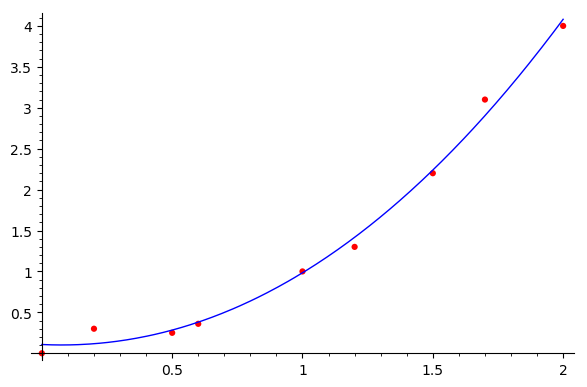
data = [(0,0), (0.2,0.3), (0.5,0.25), (0.6,0.36), 
        (1,1), (1.2, 1.3), (1.5,2.2), (1.7,3.1), (2,4)]
# Computation of a fitting polynomial of degree <=3
basis = vector([1, x, x^2, x^3])
A = matrix(len(data),len(basis),
           [basis.subs(x=datum[0]) for datum in data])
b = vector([datum[1] for datum in data])
coefs = (transpose(A)*A)\(transpose(A)*b)
f(x) = coefs*basis
# Plot results
abcissae = [datum[0] for datum in data]
x1, x2 = min(abcissae), max(abcissae)
pl = plot(f(x), (x, x1, x2))
pl += points(data, color="red", size=20)
show(pl)

This code yields the following plot:

Of course, in addition to polynomial interpolation or fitting, there are many other methods which can be used.

Assume that we have $n+1$ data points $(x_0,y_0),\ldots,(x_n,y_n)$, with $x_i\ne x_j$ for $i\ne j$. Then, there exists a unique polynomial $f$ of degree $\leq n$ such that $f(x_i)=y_i$ for $i=0,\ldots,n$. This is the Lagrange polynomial that interpolates the given data. In his answer, @dsejas has shown a method to compute it. In the current case, since $n=3$, the interpolating polynomial has degree $\leq3$; in fact, it is $f(x)=x^2$.

If $f(x)=a_0+a_1x+\cdots+a_nx^n$, it follows from the interpolation conditions that the coefficients are the solution of the linear system $A\mathbf{x}=\mathbf{b}$, where $A=(x_i^j)$ (the element of $A$ at row $i$ and column $j$ is $x_i^j$) $x_i^j$), $\mathbf{b}=(y_i)$ and $\mathbf{b}=(y_i)$. $\mathbf{x}$ is the vector of unknowns $a_0,\ldots,a_n$. This is not the best way to get $a_0,\ldots,a_n$, since $A$ is usually an ill conditioned matrix. However, it is interesting to point out that from a theoretical viewpoint.

If one has $m$ data points and still wants to fit them using a polynomial of degree $n$, with $n\leq m$, the linear system $A\mathbf{x}=\mathbf{b}$ is overdetermined (there are more equations than unknowns). In such a case, one can perform a least squares fitting, trying to minimize the interpolation errors, that is, one seeks for the minimum of $$E(a_0,a_1,\ldots,a_n)=\sum_{i=0}^m (f(x_i)-y_i)^2.$$ The minimum is given by the solution of the linear system $$ \nabla E(a_0,a_1,\ldots,a_n)=\mathbf{0},$$ which is simply $A^TA\mathbf{x}=A^T\mathbf{b}$. This is what @Cyrille, in fact, proposes in his answer... computing explicitly $E(a_0,a_1,\ldots,a_n)$ as well as its partial derivatives, which is completely unnecessary. In fact, if the system $A\mathbf{x}=\mathbf{b}$ has a unique solution, which is the case under discussion, the system $A^TA\mathbf{x}=A^T\mathbf{b}$ yields exactly the same solution. So, the function in @Cyrille's answer is just the Lagrange polynomial already proposed by @dsejas.

There are functions to compute least squares approximations in libraries like Scipy. Anyway, for such a simple case as that considered here, the following (suboptimal) code may work. Please note that I have added some points to make the example a bit more interesting:

# Data
data = [(0,0), (0.2,0.3), (0.5,0.25), (0.6,0.36), 
        (1,1), (1.2, 1.3), (1.5,2.2), (1.7,3.1), (2,4)]
# Computation of a fitting polynomial of degree <=3
basis = vector([1, x, x^2, x^3])
A = matrix(len(data),len(basis),
           [basis.subs(x=datum[0]) for datum in data])
b = vector([datum[1] for datum in data])
coefs = (transpose(A)*A)\(transpose(A)*b)
f(x) = coefs*basis
# Plot results
abcissae = [datum[0] for datum in data]
x1, x2 = min(abcissae), max(abcissae)
pl = plot(f(x), (x, x1, x2))
pl += points(data, color="red", size=20)
show(pl)

This code yields the following plot:

Of course, in addition to polynomial interpolation or fitting, there are many other methods which can be used.