Revision history [back]

Very interesting graph.

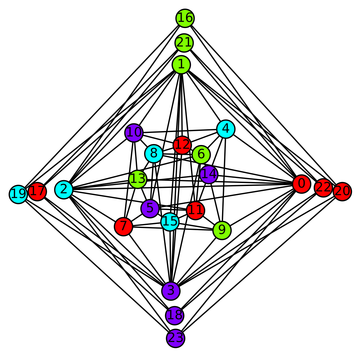
Just want to complement @vdelecroix's answer. For this purpose the graph has been redrawn (and relabeled as a side effect, sorry!). Here is the new definition of the graph together with the positions for vertices.

g = Graph({0:[1,2,3,4,5,8,9,13,14,16,18,21,23],1:[0,2,3,4,5,10,11,12,15,17,19,20,22],2:[0,1,3,6,7,10,11,13,14,16,18,21,23],3:[0,1,2,6,7,8,9,12,15,17,19,20,22],4:[0,1,6,9,10,12,14],5:[0,1,7,8,11,13,15],6:[2,3,4,8,11,12,14],7:[2,3,5,9,10,13,15],8:[0,3,5,6,10,12,13],9:[0,3,4,7,11,14,15],10:[1,2,4,7,8,12,13],11:[1,2,5,6,9,14,15],12:[1,3,4,6,8,10],13:[0,2,5,7,8,10],14:[0,2,4,6,9,11],15:[1,3,5,7,9,11],16:[0,2,19,20],17:[1,3,18,21],18:[0,2,17,22],19:[1,3,16,23],20:[1,3,16,23],21:[0,2,17,22],22:[1,3,18,21],23:[0,2,19,20]}); g.set_pos({0:[304,171],1:[177,297],2:[53,165],3:[166,58],4:[224,229],5:[144,145],6:[198,202],7:[116,126],8:[148,203],9:[220,122],10:[127,225],11:[192,143],12:[178,212],13:[131,176],14:[206,181],15:[165,131],16:[181,346],17:[25,163],18:[170,32],19:[5,160],20:[347,163],21:[180,320],22:[327,167],23:[171,8]});
color_partitions = all_graph_colorings(g,4)

The way to display a colored graph is to use the partition argument from the plot method, as shown below.

cp = color_partitions.next()
g.show(partition=cp)

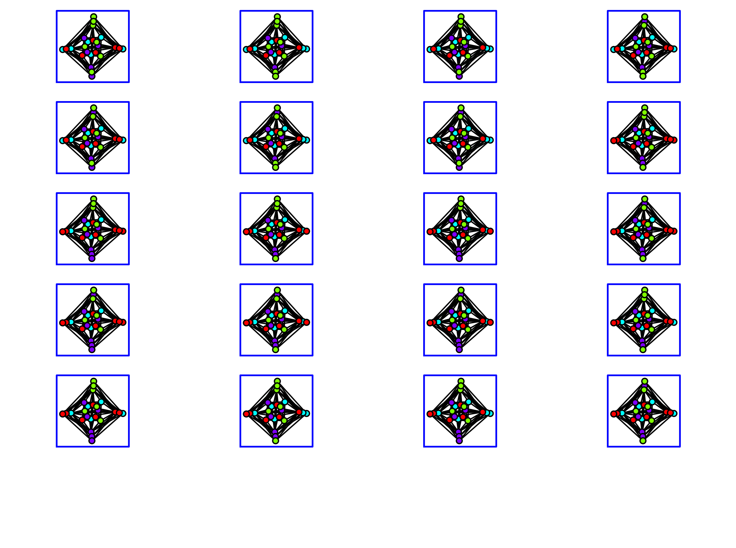
Now, if you wish to display several colorings, here is a slight modification of the graphs_list.to_graphics_array method that allows you to display them (this could possibly be further tweaked to get better pictures though).

def plot_next_few_colorings(g,color_partition_iterator,nframes=20):
    plist = []
    for i,color_partition in enumerate(color_partition_iterator):
        plist.append(g.plot(vertex_size=20,partition=cp, vertex_labels=False, graph_border=True))
        if i==nframes-1:
            break
    return graphics_array(plist, ncols=4)

Then plot_next_few_colorings(g,color_partitions) should produce a plot similar to the one shown below.