Ask Your Question
1

Implicit plot with complex function

asked 2020-12-19 23:44:26 +0200

updated 2020-12-20 12:38:23 +0200

I have a complex function $f:\mathbb{C}\to\mathbb{C}$ and want to draw the locus where $f$ is in the interval $[0,1]$.

I made the following (where $f$ is my complex function):

x = var('x')
assume(x, 'real')
y = var('y')
assume(y, 'real')
F = f.subs(z == x + I*y)
P = lambda x, y: F.subs(x=x, y=y).real()
Q = lambda x, y: F.subs(x=x, y=y).imag()
region_plot([P(x, y) <= 1, P(x, y) >= 0, Q(x, y) == 0], (x, 0, 5), (y, -1, 1))

That works well for small functions (low degree) but for big functions it's too long. For example with $$ f(z)=-\frac{{\left(z^{4} - 6 z^{3} + 12 z^{2} - 8 \, z\right)} {\left(z - 1\right)}^{3} {\left(z - 3\right)}}{{\left(2z - 3\right)} {\left(z - 2\right)}^{3} z} $$ there is no problem (a few second), but with $$ f(z)=-\frac{{\left(z^{8} - 16 z^{7} + 108 z^{6} - 400 z^{5} + 886 z^{4} - 1200 z^{3} + 972 z^{2} - 432 z + 81\right)} {\left(z - 2\right)}^{6} {\left(z - 4\right)} z}{{\left(6 z^{4} - 48 z^{3} + 140 z^{2} - 176 z + 81\right)} {\left(z - 1\right)}^{4} {\left(z - 3\right)}^{4}} $$ that's too long. I think there should be something better. I've seen for example the function complex_plot works well even for big functions and seems to do something more complex.

Any idea?

edit retag flag offensive close merge delete

Comments

Welcome to Ask Sage! Thank you for your question!

Ideally, to get answerers started, add some examples of $f$ that one can copy-paste to explore.

Maybe one example for which this works well, and one for which it does not.

slelievre gravatar imageslelievre ( 2020-12-20 01:58:23 +0200 )edit

Thanks for your help, I added some examples.

Gabriel Soranzo gravatar imageGabriel Soranzo ( 2020-12-20 13:01:43 +0200 )edit
1

Thanks for adding in examples. That seems to have inspired great answers!

slelievre gravatar imageslelievre ( 2020-12-23 20:27:54 +0200 )edit

2 Answers

Sort by » oldest newest most voted
4

answered 2020-12-22 00:41:45 +0200

Juanjo gravatar image

updated 2020-12-24 16:25:51 +0200

slelievre gravatar image

Given a function $f:\mathbb{C}\to\mathbb{C}$, the objective is to plot the set $$R=\{z\in\mathbb{C} \mid f(z)\in[0,1]\},$$ or, equivalently, $$S=\{(x,y)\in\mathbb{R}^2 \mid 0\leq P(x,y) \leq 1, \ Q(x,y)=0\},$$ where $P(x,y)$ and $Q(x,y)$ are, repectively, the real and the imaginary parts of $f(x+ i\,y)$.

In the approach followed in the original post, the bottleneck is the evaluation of the symbolic expression F, which is equal to $f(x+i\,y)$. To speed up computations, we can use the function fast_callable in order to transform F into a bivariate function that can be quickly evaluated:

var("x,y,z")
num = -(z^4-6*z^3+12*z^2-8*z)*(z-1)^3*(z-3) 
den = (2*z-3)*(z-2)^3*z
f = num/den
F = fast_callable(f.subs(z == x + I*y), vars=[x,y], domain=CDF)

Now F behaves as a bivariate function which yields complex numbers, using floating point arithmetic. For example,

 sage: F(1,2)
 -2.8235294117647056 + 4.705882352941177*I

We next define P and Q, and plot the set $S$:

P = lambda x, y: F(x,y).real()
Q = lambda x, y: F(x,y).imag()
threshold = 5e-3
S = lambda x, y: 0 <= P(x,y) <= 1 and abs(Q(x,y)) < threshold
pS = region_plot(S, (x, 0, 5), (y, -1, 1), plot_points=501,
                incol="lightgreen", bordercol="darkgreen")
show(pS, frame=True, axes=False)

The result is

Preimage of the unit interval under a rational map

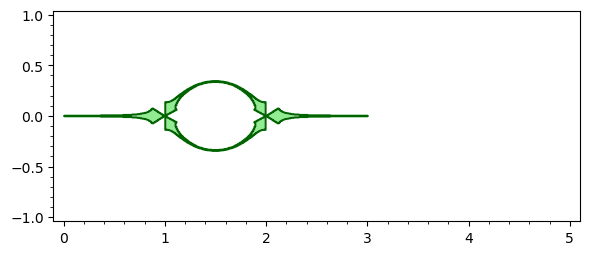
Observe that, since we are using floating point arithmetic, a condition like Q(x,y)==0 does not work, due to rounding errors. So we have replaced it by abs(Q(x,y)) < threshold. Likewise, a large number of plot points is required to get a visually smooth region. Even so, the image is not satisfactory, so let us explore a different approach.

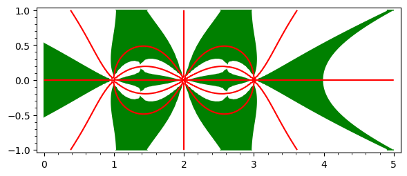
Instead of region_plot, we now use contour_plot and implicit_plot to draw, respectively, the region associated to the constraint $0\leq P(x,y)\leq 1$ and the curve $Q(x,y)=0$. Then we superimpose both plots:

pP = contour_plot(P, (0, 5), (-1, 1), contours=[0,1], 
                  plot_points=101, cmap=["white","green","white"])
pQ = implicit_plot(Q, (0, 5), (-1, 1), color="red")
show(pP+pQ)

Preimage of the unit interval under a rational map

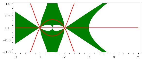
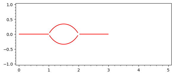
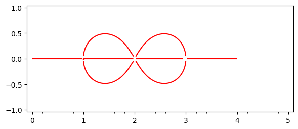
Hence $S$ is the set of red lines on the green background, quite similar, by the way, to the set shown in the first picture. Can we isolate those red lines? Yes, by using the region option:

implicit_plot(Q, (0, 5), (-1, 1), region=lambda x,y: 0<= P(x,y) <= 1, 
              plot_points=201, color="red")

Preimage of the unit interval under a rational map

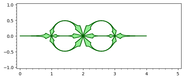
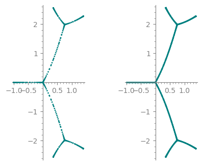
Up to now we have dealt with the first function $f$ given in the OP. For the second one, it suffices to change num and den as follows:

num = -(z^8 -16*z^7+108*z^6-400*z^5+886*z^4-1200*z^3+972*z^2-432*z+81)*(z-2)^6*(z-4)*z
den = (6*z^4-48*z^3+140*z^2-176*z+81)*(z-1)^4*(z-3)^4

And then repeat all the steps. We get the following pictures:

Preimage of the unit interval under a rational map

Preimage of the unit interval under a rational map

Preimage of the unit interval under a rational map

The complete code for the second case can be seen in this SageMathCell.


The above code for "implicit plot of Im = 0 in the region 0 <= Re <= 1" as a function:

def pre01_line(f, xx=(0, 4), yy=(-1, 1), **opt):
    r"""
    Return the preimage of the unit interval under this map.

    INPUT:

    - ``f`` -- a complex map as a symbolic expression

    - ``xx``, ``yy`` -- the range of ``x`` and ``yy`` where to plot
    """
    z = f.variables()[0]
    x, y = SR.var('x, y')
    F = fast_callable(f.subs({z: x + I*y}), vars=[x, y], domain=CDF)
    P = lambda x, y: F(x, y).real()
    Q = lambda x, y: F(x, y).imag()
    op = {'region': lambda x, y: 0 <= P(x, y) <= 1,
          'plot_points': 129, 'color': 'red'}
    for k, v in op.items():
        if k not in opt:
            opt[k] = v
    p = implicit_plot(Q, xx, yy, **opt)
    return p

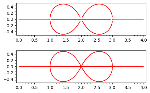
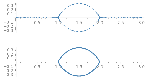
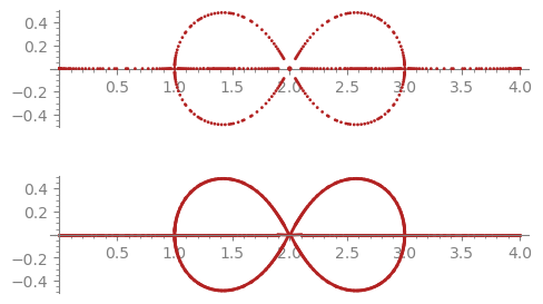
Lines don't quite meet in some places (a tighter bounding box improves things though):

num = -(z^8 -16*z^7+108*z^6-400*z^5+886*z^4-1200*z^3+972*z^2-432*z+81)*(z-2)^6*(z-4)*z
den = (6*z^4-48*z^3+140*z^2-176*z+81)*(z-1)^4*(z-3)^4
f = num/den
a = pre01_line(f, xx=(0, 4), yy=(-0.5, 0.5))
a.show()

Increasing the number of plot points on the whole figure would be computationally wasteful.

Instead, why not simply fill in the small missing patches:

b = sum((pre01_line(f, xx=(k - eps, k + eps), yy=(-eps, eps), plot_points=65)
         for k in (1, 2, 3) for eps in [1/16]), a)
b.show()

Compare the two plots:

ab = graphics_array([a, b], ncols=1)
ab.show(transparent=True, figsize=5)

Preimage of the unit interval under a rational map

edit flag offensive delete link more

Comments

@slelievre, many thanks for your edit, which really improves the answer.

Juanjo gravatar imageJuanjo ( 2020-12-25 23:26:16 +0200 )edit
3

answered 2020-12-21 10:57:45 +0200

FrédéricC gravatar image

updated 2020-12-24 10:46:57 +0200

Are you working on dessins d'enfants?

Here is a simple idea for an approximate plot.

sage: x = polygen(QQ, 'x')                                           
sage: f = 1/729*(2*x**2-3*x+9)**3*(x+1)                           
sage: N = 50               
sage: point2d(root for k in range(N+1) for root in (f - k / N).complex_roots())

Quick example: preimage of unit interval under rational function

The function pre01 below builds on this idea. It gives a good idea of the desired plot and runs fast.

def pre01(f, n=50, style='dots', **opt):
    r"""
    Return the preimage of the unit interval under this rational function.

    INPUT:

    - ``f`` -- a rational function

    - ``n`` -- optional (default: 50) -- roughly how many points
      in the unit interval [0, 1] to use for preparing the plot

    Roughly a third or the points are inverse powers of two,
    roughly a third are one minus inverse powers of two,
    and roughly a third are linearly spaced along the interval.

    EXAMPLES::

        sage: x = polygen(QQ, 'x')
        sage: f = 1/729 * (2 * x**2 - 3 * x + 9)**3 * (x + 1)
        sage: pre01(f, n=50, style='dots', color='firebrick').show(figsize=5)
        sage: pre01(f, n=50, style='line', color='firebrick').show(figsize=5)

        sage: z = polygen(QQ, 'z')
        sage: num = -(z^4-6*z^3+12*z^2-8*z)*(z-1)^3*(z-3) 
        sage: den = (2*z-3)*(z-2)^3*z
        sage: g = num/den
        sage: pre01(g, n=50, style='dots', color='firebrick').show(figsize=5)
        sage: pre01(g, n=50, style='line', color='firebrick').show(figsize=5)

        sage: Qz.<z> = QQ[]
        sage: cc = [81, -432, 972, -1200, 886, -400, 108, -16, 1]
        sage: num = -Qz(cc)*(z-2)^6*(z-4)*z
        sage: den = (6*z^4-48*z^3+140*z^2-176*z+81)*(z-1)^4*(z-3)^4
        sage: h = num/den
        sage: pre01(h, n=50, style='dots', color='firebrick').show(figsize=5)
        sage: pre01(h, n=50, style='line', color='firebrick').show(figsize=5)
    """
    nn = n // 3 + 2
    num, den = f.numerator(), f.denominator()
    tt = [0] + [ZZ(2)**-k for k in (0 .. nn)]
    tt.extend([1 - t for t in tt[3:]])
    tt.extend(QQ((k, nn)) for k in (1 .. nn - 1))
    tt = sorted(set(tt))
    cols = {'color': 'teal', 'axes': True, 'axes_color': 'grey',
            'axes_label_color': 'grey', 'tick_label_color': 'grey'}
    dop = {'aspect_ratio': 1, 'size': 4, 'zorder': 10}
    lop = {'aspect_ratio': 1, 'edge_thickness': 2}
    for k, v in opt.items():
        if 'color' in k or 'axis' in k or 'axes' in k or 'tick' in k:
            cols[k] = v
        elif k == 'size':
            dop[k] = v
        elif k == 'edge_thickness':
            lop[k] = v
        else:
            dop[k] = lop[k] = v
    if style == 'dots':
        zz = (root for t in set(tt) for root in (num - t*den).complex_roots())
        G = point2d(zz, color=cols['color'], **dop)
    elif style == 'line':
        tzz = {t: (num - t*den).complex_roots() for t in tt}
        D = Graph()
        for k, t in enumerate(tt[1:-1], start=1):
            s, u = tt[k-1], tt[k+1]
            szz, uzz = tzz[s], tzz[u]
            for z in tzz[t]:
                zs = min((abs(z - w), w) for w in szz)[1]
                D.add_edge(z, zs, k-1)
                zu = min((abs(z - w), w) for w in uzz)[1]
                D.add_edge(z, zu, k)
        D.set_pos({z: (z.real(), z.imag()) for z in D})
        ecol = {cols['color']: D.edges()}
        G = D.plot(vertex_labels=False, vertex_size=0, edge_colors=ecol, **lop)
    else:
        raise ValueError(f"style should be 'dots' or 'line', got :'{style}'")
    G.axes(cols['axes'])
    G.axes_color(cols['axes_color'])
    G.axes_label_color(cols['axes_label_color'])
    G.tick_label_color(cols['tick_label_color'])
    return G

Three examples of using this function follow.

Quick starting example of this answer:

x = polygen(QQ, 'x')
f = 1/729 * (2 * x**2 - 3 * x + 9)**3 * (x + 1)
a_dots = pre01(f, n=50, style='dots', color='teal')
a_line = pre01(f, n=50, style='line', color='teal')
a_dots_lines = graphics_array([a_dots, a_line], ncols=2)
a_dots_lines.show(figsize=5)

Preimage of unit interval under map f

First example in the question:

z = polygen(QQ, 'z')
num = -(z^4-6*z^3+12*z^2-8*z)*(z-1)^3*(z-3) 
den = (2*z-3)*(z-2)^3*z
b_dots = pre01(num/den, n=50, style='dots', color='steelblue')
b_line = pre01(num/den, n=50, style='line', color='steelblue')
b_dots_lines = graphics_array([b_dots, b_line], ncols=1)
b_dots_lines.show(figsize=5)

Preimage of unit interval under first map in question

Second example in the question:

z = polygen(QQ, 'z')
num = -(z^8-16*z^7+108*z^6-400*z^5+886*z^4-1200*z^3+972*z^2-432*z+81)*(z-2)^6*(z-4)*z
den = (6*z^4-48*z^3+140*z^2-176*z+81)*(z-1)^4*(z-3)^4
c_dots = pre01(num/den, n=50, style='dots', color='firebrick')
c_line = pre01(num/den, n=50, style='line', color='firebrick')
c_dots_lines = graphics_array([c_dots, c_line], ncols=1)
c_dots_lines.show(figsize=5)

Preimage of unit interval under second map in question

Each of those three examples runs in under a second per plot style.

edit flag offensive delete link more

Comments

Yes, I'm working on Dessins d'enfants. You too? I would be interested in knowing in what laboratory you're working... we are so few to work on it!

Gabriel Soranzo gravatar imageGabriel Soranzo ( 2022-06-11 15:24:02 +0200 )edit

Your Answer

Please start posting anonymously - your entry will be published after you log in or create a new account.

Add Answer

Question Tools

1 follower

Stats

Asked: 2020-12-19 23:44:26 +0200

Seen: 682 times

Last updated: Dec 24 '20