Ask Your Question
1

Defining a function with different symbolic expressions in different parts of its domain specified by conditional statements

asked 2020-10-17 19:31:09 +0200

Shaolinux gravatar image

updated 2020-10-18 04:51:33 +0200

I am struggling with a definition of a functional surface z=z(x,y) where z is positive in the interior of a triangle, zero on its boundary, and zero outside of it everywhere on a rectangle for (x,y) which contains the triangle. All necessary formulae can be provided in if/elif/else/return, etc. statements. Yet, I get errors when using def and return (I have never worked with simpy and would prefer to avoid using lambdas and stay as close to the mathematical expressions as possible). I think that if someone helps with explaining how to handle a simple definition of a 1-variate function of x=var('x'), I'll figure what I am not doing right also in the 2-variate case x, y = var('x,y'). So here is a very simple example:

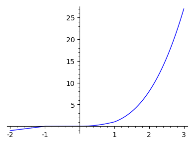
f has definition domain -2<=x<=3 and is defined with different formulae on different parts of its domain, e.g.,

f(x)=x+1 when x is between -2 and -1,

f(x)=0 when x is between -1 and 0,

f(x)=x^2 when x is between 0 and 1,

f(x)=x^3 when x is between 1 and 3,

(naturally, without overlapping at the boundaries, although this function is continuous there, so no problems arise there -- I skipped the use of inequalities because the preview program got confused).

After the definition I would like to use f(x) while specifying for x the WHOLE range [-2,+3]. (For example, plot the graph of y=f(x) for all x between -2 and +3.) Can someone please provide a simple working code, say, using def and conditional statements but not resorting to tuples, classes (ok, if there is absolutely not a simple way, lambdas can be used as a last resort :) )? Or maybe this question has been answered earlier? Please help :)

Following the fairly exhaustive answers of rburing and tmonteil below to the 1-variate version of my question, I now proceed to upgrading it for 2-variate functions with a maximally simplified concrete problem which, if solved, can immediately be upgraded also to the 3-variate case. (In the formulation, I shall use latex notation.)

Consider the square domain (x,y) \in A=[-2,2]x[-2,2] and a subset of its interior: the 'canonical' triangle B with vertices P_0=O=(0,0), P_1=(1,0) and P_2=(0,1). The reason for this 'canonical' choice is that the cartesian coordinates x and y coincide with two of the three barycentric coordinates of an arbitrary point P in the plane Oxy: P=(x,y)=(1-x-y).P_0+x.P_1+y.P_2; moreover, if P is in B or on its boundary, then the combination is CONVEX; (moreover, if P is on the interior of an edge of the boundary of B, then 1 of the three coefficients is 0, and if it is coincides with one of the vertices, then 2 of these coefficients are 0). Now I proceed to define mathematically the needed functional surface z=z(x,y), as follows:

Consider first a point P_3=(x_3, y_3) which lies in the interior of B, i.e. all the three coefficients 1-x-y, x and y are strictly positive and strictly less than 1.

if 1-x-y leq 0 or x leq 0 or y leq 0 (this is exactly the case when P=(x,y) is outside of B or lies on its boundary), then z(x,y)=0;

elsewhere on A (i.e., exactly when P lies in the interior of B), define z(x,y)=exp{-[(x-x_3)^2+(y-y_3)^2]/[(1-x-y)^2(x^2)(y^2)]}.

Now z(x,y) is defined on the whole A and has several remarkable properties there. As a non-exhaustive example:

it is analytic everywhere on A except the boundary of B where it is still C^\infty - smooth but not analytic (the Taylor expansion series is not convergent there, but is convergent everywhere else on A).

it takes strictly positive values less than 1 (good as coefficient in a convex combination!) and reaches its global maximum equal to 1 exctly and only in the prescribed point P_3.

To define this type of functional surface on an arbitrary triangle in Oxy or as a parametric surface in 3D one now uses a standard approach (used in finite/boundary element theory, geometric design, etc, etc.) via applying a non-singular affine transformation. The technique is easy to extend to tetrahedra in 3D.

To explain why this function has numerous prospective valuable applications is a very long story. To cut it short, I promise that if you help solve this particular problem, you will soon read about some of its new applications in the newspapers... :) :) :)

Summarizing:

the primary, maximally simplified, task I ask to be solved here is to provide SageMath (Python 3) code to use parametric_plot3d to plot the parametric surface X(u,v)=u, Y(u,v)=v, Z(u,v)=z(u,v) for (u,v) in the parametric domain A given above and to view it in Ubuntu using threejs and/or jmol. (Forget about all the extra options, Windows limitations, etc).

Can you help, please?

edit retag flag offensive close merge delete

Comments

May I suggest refraining from reinventing the wheel and looking up Wikipedia and linked pages ?

Emmanuel Charpentier gravatar imageEmmanuel Charpentier ( 2020-10-18 14:27:30 +0200 )edit

Point taken. In the future I shall refrain from joking at the forum and I suggest that you refrain from joking, too.

Shaolinux gravatar imageShaolinux ( 2020-10-19 01:57:46 +0200 )edit

3 Answers

Sort by ยป oldest newest most voted
0

answered 2020-10-18 00:03:06 +0200

tmonteil gravatar image

You can define a piecewise symbolic function, see https://doc.sagemath.org/html/en/refe...

edit flag offensive delete link more

Comments

I thank also tmonteil for providing this valuable addition to the answer of rburing above, and especially for the cited link which promises to be helpful in many ways. Everything which I wrote in my remark to rburing's answer above is valid, mutatis mutandis, also for this answer.

I will now proceed to upgrade my question above to the case of 2D. A successful solution will have applications to triangulation techniques for 2D domains for parametric surfaces and will almost certainly be possible to extend straightforwardly to tetrahedralization techniques for 3D domains, 3D-volume deformations, scalar and vector-field visualization in 3D and other issues which are likely to be of general interest for diverse parts of the SageMath user communty.

Shaolinux gravatar imageShaolinux ( 2020-10-18 03:11:08 +0200 )edit
1

answered 2020-10-18 00:37:53 +0200

rburing gravatar image

updated 2020-10-18 11:59:52 +0200

If your goal is to plot, then you only need a function that accepts numbers and returns numbers:

def f(x):
    if -2 <= x < -1:
        return x + 1
    elif -1 <= x < 0:
        return 0
    elif 0 <= x < 1:
        return x^2
    elif 1 <= x <= 3:
        return x^3

Indeed,

sage: plot(f,(-2,3))

piecewise plot

Now, this function does not play well with symbolic variables:

sage: var('x')
sage: print(f(x))
None

It is because inequalities with symbolic variables only evaluate to True when Sage can prove them; here none of them can be proved because nothing is known about x. If you add assumptions then you can achieve something:

sage: assume(0<=x)
sage: assume(x<1)
sage: f(x)
x^2

But it does not help with plotting. The above explains why e.g. var('x'); plot(f(x),(x,2,3)) does not work.

You can have univariate piecewise-defined symbolic functions in Sage, to some extent:

sage: var('x')
sage: f = piecewise([([-2,-1], x+1), ((-1,0), 0), ((0,1), x^2), ([1,3], x^3)])
sage: plot(f,(-2,3))

It gives the same plot. Now it is also possible to evaluate f(x) for symbolic x:

sage: f(x)
piecewise(x|-->x + 1 on [-2, -1], x|-->0 on (-1, 0), x|-->x^2 on (0, 1), x|-->x^3 on [1, 3]; x)
sage: plot(f(x),(x,-2,3))

Again, the same plot. This 'piecewise' functionality is unfortunately somewhat fragile, e.g. diff(f,x) returns junk.


To plot a surface with a piecewise parametrization, avoid symbolic variables:

def g(x,y):
    if x >= y:
        return x
    else:
        return y

parametric_plot3d([lambda x,y: x, lambda x,y: y, g], (-1,1), (-1,1))

Your surface:

x_3, y_3 = 1/3, 1/4

def X(u,v):
    return u
def Y(u,v):
    return v
def Z(u,v):
    if 1-u-v <= 0 or u <= 0 or v <= 0: # when P=(u,v) is outside of B or lies on its boundary
        return 0
    else: # i.e., exactly when P lies in the interior of B
        return exp(-((u-x_3)^2+(v-y_3)^2)/((1-u-v)^2*(u^2)*(v^2)))

print(Z(x_3,y_3))
parametric_plot3d([X,Y,Z], (x_3-0.1,x_3+0.1), (y_3-0.1,y_3+0.1), plot_points=[200,200], viewer='threejs')
parametric_plot3d([X,Y,Z], (-2,2), (-2,2), plot_points=[200,200], viewer='threejs')
edit flag offensive delete link more

Comments

I thank rburing for providing this valuable shortcut in my education in SageMath. I shall study carefully all of the above variants and now have confidence that the problem about defining and processing piecewise-defined 1-variate functions (hence, also parametric curves in 3D) is essentially resolved (point taken, concerning the specifics of the range of applications of numpy vs. sympy). I am still new here and do not have the needed points yet to mark the question as answered but will certainly do so when I have the necessary number of points.

This rapidly provided comprehensive solution gives me hope that with the help of asksage community will be resolved also the 2D problem I am facing now. So, after posting this remark, I shall upgrade my question to include also the 2D problem.

Shaolinux gravatar imageShaolinux ( 2020-10-18 02:49:13 +0200 )edit
1

answered 2020-10-19 01:50:46 +0200

Shaolinux gravatar image

updated 2020-10-19 02:07:08 +0200

This is a report on the updated question after the replies by rburing and tmonteil.

The answer and recommendations of rburing concerning the 1-variate example worked beautifully also for the newly proposed 2D example, as follows:

x, y = var('x,y')
def f(x,y):    
    if -2.<=x<=0.:
        return 0.
    elif -2.<=y<=0.:
        return 0.
    elif 1-x-y<=0.:
        return 0.
    elif 1.<=x<=2.:
        return 0.
    elif 1.<=y<=2.:
        return 0.
    else:
        return 0.1*exp(-0.01*((x-1/3)^2+(y-1/3)^2)/(((1-x-y)^2)*(x^2)*(y^2)))
def g(x,y):
    return x
def h(x,y):
    return y
P=parametric_plot3d([g, h, f], (x, -2, 2), (y, -2, 2), plot_points=[128,128], frame=False, color="silver", opacity=1.)
P.show(viewer='threejs')

This is solving completely the part of the problem of plotting the graph. However, the use of conditional statements yielded the graph on the whole rectangle [-2,2]^2. Although we have used x and y as barycentric coordinates here, this is still not convenient to be used as a triangular patch.

The following is a suggestion how to resolve this difficulty WITHOUT ANY USE OF CONDITIONAL STATEMENTS, by using reparametrization instead.

After a Jacobi change of variables for the triangle,

x=s(1-t), y=st

the triangle is reparametrized, with the square (s,t) \in [0,1]^2 being the new parametric domain. In the new variables, the expression in the 'else' statement above becomes

0.1exp(-0.01((1-t-1/(3.s))^2+(t-1/(3.s))^2)/(((1-s)^2)(s^2)((1-t)^2)*(t^2)))

and there follows the new code (this time including also s and t coordinate lines):

s, t = var('s,t')
def F(s,t):
    return 0.1*exp(-0.01*((1-t-1/(3.*s))^2+(t-1/(3.*s))^2)/(((1-s)^2)*(s^2)*((1-t)^2)*(t^2)))
def G(s,t):
    return s*(1-t)
def H(s,t):
    return s*t
Q0=parametric_plot3d([G, H, F], (s, 0, 1), (t, 0, 1), plot_points=[128,128], frame=False, color="gray", opacity=1.)
eps=0.001
M=64
N=64
L=128
m=var('m', domain='integer')
n=var('n', domain='integer')
curve3dplot_uline=[0 for i in range(M)] 
curve3dplot_vline=[0 for j in range(N)]
curve3dplot_uline=[parametric_plot3d([G(s,eps+m*(1.-2.*eps)/M), H(s,eps+m*(1.-2.*eps)/M), F(s,eps+m*(1.-2.*eps)/M)],  (s, 0, 1), plot_points=128, color='silver', thickness=.5, opacity=1.) for m in range(M)] 
curve3dplot_vline=[parametric_plot3d([G(eps+n*(1.-2.*eps)/N,t), H(eps+n*(1.-2.*eps)/N,t), F(eps+n*(1.-2.*eps)/N,t)],  (t, 0, 1), plot_points=128, color='silver', thickness=.5, opacity=1.) for n in range(N)]
Q1=sum(curve3dplot_uline[i] for i in range(M)) 
Q2=sum(curve3dplot_vline[j] for j in range(N))
Q=Q0+Q1+Q2
Q.show(viewer='threejs')

In this solution all conditional statements have been eliminated, the resulting graph is the graph of a parametric triangular patch. Many years ago, underflow error would have been reported at the boundary of the triangle, but numpy handles the exception well and interprets the value as 0., as needed. However, the computation of the coordinate s- and t-lines requires the introduction of a small positive parameter eps; otherwise, if eps=0, the result will be error of symbolic division by zero.

This construction by parametrization avoiding the use of conditional constraints can be straightforwardly generalized for a tetrahedron in 3D (and generally for a simplex in n-dimensions, n=2,3,4,...) . The needed generalization of the Jacobi reparametrization to n-dimensional simplex is well known (see, e.g. the 3rd volume of Fihtenholz).

edit flag offensive delete link more

Your Answer

Please start posting anonymously - your entry will be published after you log in or create a new account.

Add Answer

Question Tools

1 follower

Stats

Asked: 2020-10-17 19:31:09 +0200

Seen: 985 times

Last updated: Oct 19 '20