Yes one can use bipolar coordinates in SageMath provided that one sets by hand the relations between bipolar and Cartesian coordinates, as follows. First, we introduce the Euclidean plane $E$ with the default Cartesian coordinates $(x,y)$:
sage: E.<x,y> = EuclideanSpace()
sage: CA = E.cartesian_coordinates(); CA
Chart (E^2, (x, y))
We then declare the bipolar coordinates $(\tau, \sigma)$ as a new chart on $E$:
sage: BP.<t,s> = E.chart(r"t:\tau s:\sigma:(-pi,pi)")
sage: BP
Chart (E^2, (t, s))
sage: BP.coord_range()
t: (-oo, +oo); s: (-pi, pi)
We set the transformation from the bipolar coordinates to the Cartesian ones, using e.g. the Wikipedia formulas. This involves $\cosh\tau$ and $\sinh\tau$. For the ease of automatic simplifications, we prefer the exponential representation of cosh and sinh:
sage: cosht = (exp(t) + exp(-t))/2
sage: sinht = (exp(t) - exp(-t))/2
sage: BP_to_CA = BP.transition_map(CA, [sinht/(cosht - cos(s)), sin(s)/(cosht - cos(s))])
sage: BP_to_CA.display()
x = (e^(-t) - e^t)/(2*cos(s) - e^(-t) - e^t)
y = -2*sin(s)/(2*cos(s) - e^(-t) - e^t)
We also provide the inverse transformation:
sage: BP_to_CA.set_inverse(1/2*ln(((x+1)^2 + y^2)/((x-1)^2 + y^2)),
....:                      pi - 2*atan(2*y/(1-x^2-y^2+sqrt((1-x^2-y^2)^2 + 4*y^2))))
sage: BP_to_CA.inverse().display()
t = 1/2*log(((x + 1)^2 + y^2)/((x - 1)^2 + y^2))
s = pi - 2*arctan(-2*y/(x^2 + y^2 - sqrt((x^2 + y^2 - 1)^2 + 4*y^2) - 1))
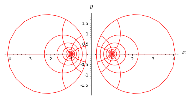
At this stage, we may plot the grid of bipolar coordinates in terms of the Cartesian coordinates (the plot is split in 2 parts to avoid $\tau = 0$):
sage: BP.plot(CA, ranges={t: (-4, -0.5)}) + BP.plot(CA, ranges={t: (0.5, 4)})
Let us do some calculus with bipolar coordinates. The Euclidean metric is
sage: g = E.metric()
sage: g.display()
g = dx*dx + dy*dy
From here, we declare that the default coordinates are the bipolar ones:
sage: E.set_default_chart(BP)
sage: E.set_default_frame(BP.frame())
We have then:
sage: g.display()
g = -4*e^(2*t)/(4*cos(s)*e^(3*t) - 2*(2*cos(s)^2 + 1)*e^(2*t) + 4*cos(s)*e^t - e^(4*t) - 1) dt*dt
     - 4*e^(2*t)/(4*cos(s)*e^(3*t) - 2*(2*cos(s)^2 + 1)*e^(2*t) + 4*cos(s)*e^t - e^(4*t) - 1) ds*ds
Let us factor the metric coefficients to get a shorter expression:
sage: g[1,1].factor()
4*e^(2*t)/(2*cos(s)*e^t - e^(2*t) - 1)^2
sage: g[2,2].factor()
4*e^(2*t)/(2*cos(s)*e^t - e^(2*t) - 1)^2
sage: g.display()
g = 4*e^(2*t)/(2*cos(s)*e^t - e^(2*t) - 1)^2 dt*dt
  + 4*e^(2*t)/(2*cos(s)*e^t - e^(2*t) - 1)^2 ds*ds
We can check the identity (cf. the Wikipedia page):
sage: g[1,1] == 1/(cosht - cos(s))^2
True
Let us consider a generic scalar field on $E$, defined by a function $F$ of the bipolar coordinates:
sage: f = E.scalar_field({BP: function('F')(t,s)}, name='f')
sage: f.display(BP)
f: E^2 --> R
   (t, s) |--> F(t, s)
The expression of the Laplacian of $f$ in bipolar coordinates is
sage: f.laplacian().expr(BP).factor()
1/4*(2*cos(s)*e^t - e^(2*t) - 1)^2*(diff(F(t, s), t, t) + diff(F(t, s), s, s))*e^(-2*t)
Again it agrees with that given in the Wikipedia page.
The gradient of $f$ is
sage: f.gradient().display()
grad(f) = -1/4*(4*cos(s)*e^(3*t) - 2*(2*cos(s)^2 + 1)*e^(2*t) + 4*cos(s)*e^t - e^(4*t) - 1)*e^(-2*t)*d(F)/dt d/dt
         - 1/4*(4*cos(s)*e^(3*t) - 2*(2*cos(s)^2 + 1)*e^(2*t) + 4*cos(s)*e^t - e^(4*t) - 1)*e^(-2*t)*d(F)/ds d/ds
